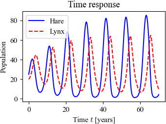
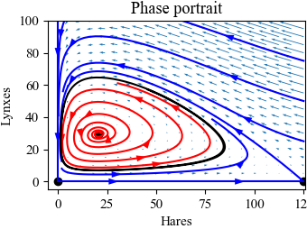
Figure 4.20: Simulation of the predator-prey system
Jump to navigation
Jump to search
| Chapter | Examples |
|---|---|
| Figure number | 4.20 |
| Figure title | Simulation of the predator–prey system |
| GitHub URL | |
| Requires | python-control, python-control |
Figure 4.20: Simulation of the predator–prey system. The figure on the left shows a simulation of the two populations as a function of time. The figure on the right shows the populations plotted against each other, starting from different values of the population. The oscillation seen in both figures is an example of a limit cycle. The parameter values used for the simulations are a = 3.2, b = 0.6, c = 50, d = 0.56, k = 125, and r = 1.6.

