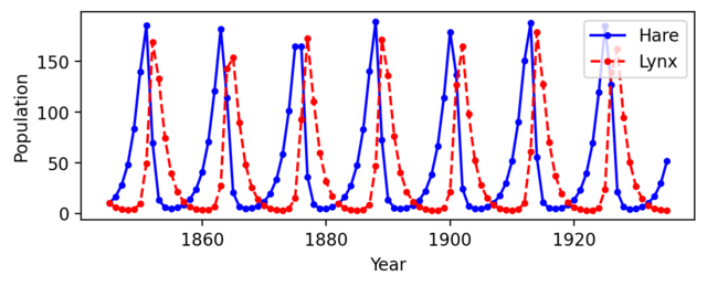
Figure 3.8: Discrete-time simulation of the predator–prey model

Chapter	System Modeling
Figure number	3.8
Figure title	Discrete-time simulation of the predator–prey model
GitHub URL	https://github.com/murrayrm/fbs2e-python/blob/main/figure-3.8-predator prey.py
Requires	python-control

Figure 3.8: Discrete-time simulation of the predator–prey model (3.13). Using the parameters $a=c=0.014$, $b_{h}(u)=0.6$, and $d_{l}=0.7$ in equation (3.13), the period and magnitude of the lynx and hare population cycles approximately match the data in Figure 3.7.

# figure-3.8-predator_prey.py - discrete-time simulation of predator–prey model
# RMM, 15 May 20219
#
# Figure 3.8: Discrete-time simulation of the predator–prey model
# (3.13). Using the parameters a = c = 0.014, bh(u) = 0.6, and dl =
# 0.7 in equation (3.13), the period and magnitude of the lynx and
# hare population cycles approximately match the data in Figure 3.7.

import control as ct
import numpy as np
import matplotlib.pyplot as plt

# Define the dynamics of the predator prey system
def predprey(t, x, u, params):
    # Parameter setup
    a = params.get('a', 0.014) / 365.
    bh0 = params.get('bh0', 0.6) / 365.
    c = params.get('c', 0.014) / 365.
    dl = params.get('dl', 0.7) / 365.
    
    # Map the states into local variable names
    H = x[0]
    L = x[1]

    # Compute the input
    bhu = bh0 + u

    # Compute the discrete updates
    dH = H + bhu * H - a * L * H
    dL = L + c * L * H - dl * L

    return [dH, dL]

# Create a nonlinear I/O system (dt = days)
io_predprey = ct.NonlinearIOSystem(
    predprey, None, inputs=('u'), outputs=('H', 'L'),
    states=('H', 'L'), name='predprey', dt=1/365)

X0 = [10, 10]                               # Initial H, L
T = np.linspace(1845, 1935, 90*365 + 1)     # 90 years

# Simulate the system
response = ct.input_output_response(io_predprey, T, 0, X0)
t, y = response.time, response.outputs

# Downsample the responses to individual years
yrs = t[::365]
pop = y[:, ::365]

# Plot the response
plt.subplot(2, 1, 1)            # Set the aspect ration to match the text

plt.plot(yrs, pop[0], 'b-o', markersize=3)
plt.plot(yrs, pop[1], 'r--o', markersize=3)
plt.legend(["Hare", "Lynx"])

plt.xlabel("Year")
plt.ylabel("Population")