System Modeling
| Prev: Feedback Principles | Chapter 3 - System Modeling | Next: Examples |
A model is a precise representation of a system’s dynamics used to answer questions via analysis and simulation. The model we choose depends on the questions we wish to answer, and so there may be multiple models for a single dynamical system, with different levels of fidelity depending on the phenomena of interest. In this chapter we provide an introduction to the concept of modeling and present some basic material on two specific methods commonly used in feedback and control systems: differential equations and difference equations.
Contents
- Modeling Concepts
- State Space Models
- Modeling Methodology
- Modeling Examples
- Further Reading
- Exercises
Chapter Summary
-
A model is a mathematical representation of a system that can be used to answer question about that system. The choice of the model depends on the questions one wants to ask. Models for control systems are typically input/output models and combine techniques from mechanics and electrical engineering.
The state of a system is a collection of variables that summarize the past history of the system for the purpose of predicting the future. A state space model is one that describes how the state of a system evolves over time.
We can model the evolution of the state using ordinary differential equations of the form
Nonlinear Linear Another class of models for feedback and control systems is a difference equation of the form
Nonlinear Linear Three common questions that can be answered using state space models are (1) how the system state evolves from a given initial condition, (2) the stability of an equilibrium point from nearby initial conditions and (3) the steady state response of the system to sinusoidal forcing at different frequencies.
Models can be constructed from experiments by measuring the response of a system and determining the parameters in the model that correspond to features in the response. Examples include measuring the period of oscillation, the rate of damping and the steady state amplitude of the response of a system to a step input.
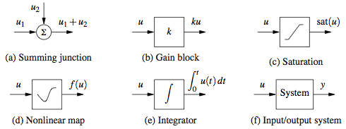
Schematic and block diagrams are common tools for modeling large, complex systems. The following symbols are some of the ones commonly used for modeling control systems:

Modeling examples (wiki-based):


