Difference between revisions of "Figure 3.24: Consensus protocols for sensor networks"
Jump to navigation
Jump to search
(Created page with "{{Figure |Chapter=System Modeling |Figure number=24 |Figure title=Consensus protocols for sensor networks |GitHub URL=https://github.com/murrayrm/fbs2e-python/blob/main/figure...") |
|||
| Line 5: | Line 5: | ||
|GitHub URL=https://github.com/murrayrm/fbs2e-python/blob/main/figure-3.24-consensus.py | |GitHub URL=https://github.com/murrayrm/fbs2e-python/blob/main/figure-3.24-consensus.py | ||
}} | }} | ||
| − | [[Image:figure-3.24-consensus_dynamics.png| | + | [[Image:figure-3.24-consensus_dynamics.png|320px]] |
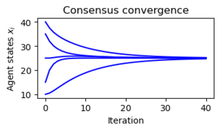
Figure 3.24: Consensus protocols for sensor networks. (b) A simulation demonstrating the convergence of the consensus protocol (3.35) to the average value of the initial conditions. | Figure 3.24: Consensus protocols for sensor networks. (b) A simulation demonstrating the convergence of the consensus protocol (3.35) to the average value of the initial conditions. | ||
Revision as of 16:23, 30 August 2021
| Chapter | System Modeling |
|---|---|
| Figure number | 24 |
| Figure title | Consensus protocols for sensor networks |
| GitHub URL | https://github.com/murrayrm/fbs2e-python/blob/main/figure-3.24-consensus.py |
| Requires | python-control |
Figure 3.24: Consensus protocols for sensor networks. (b) A simulation demonstrating the convergence of the consensus protocol (3.35) to the average value of the initial conditions.
# example-3.17-consensus.py - consensus protocols
# RMM, 30 Aug 2021

# Figure 3.24: Consensus protocols for sensor networks. (a) A simple sensor
# net- work with five nodes. In this network, node 1 communicates with node
# 2 and node 2 communicates with nodes 1, 3, 4, 5, etc. (b) A simulation
# demonstrating the convergence of the consensus protocol (3.35) to the
# average value of the initial conditions.

import control as ct
import numpy as np
import matplotlib.pyplot as plt

#
# System dynamcis
#

# Construct the Laplacian corresponding to our network
L = np.array([
    [ 1, -1,  0,  0,  0],
    [-1,  4, -1, -1, -1],
    [ 0, -1,  2, -1,  0],
    [ 0, -1, -1,  2,  0],
    [ 0, -1,  0,  0,  1]
])

# Now generate the discrete time dynamics matrix
gamma = 0.1
A = np.eye(5) - gamma * L

# Initial set of measurements for the system
x0 = [10, 15, 25, 35, 40]

# Create a discrete time system
sys = ct.ss(A, np.zeros(5), np.zeros(5), 0, dt=True)

# Set up the plotting grid to match the layout in the book
fig = plt.figure(constrained_layout=True)
gs = fig.add_gridspec(3, 2)

#
# (b) A simulation demonstrating the convergence of the consensus protocol
# (3.35) to the average value of the initial conditions.
#

fig.add_subplot(gs[0, 1])       # first row, first column

# Simulate the system
response = ct.initial_response(sys, 40, x0)

# Plot th3 results
for i in range(response.nstates):
    plt.plot(response.time, response.states[i], 'b-')

# Label the figure
plt.xlabel("Iteration")
plt.ylabel("Agent states $x_i$")
plt.title("Consensus convergence")

# Save the figure
plt.savefig("figure-3.24-consensus_dynamics.png", bbox_inches='tight')
