Difference between revisions of "Figure 5.6: Illustration of Lyapunov’s concept of a stable solution"
Jump to navigation
Jump to search
(Created page with "{{Figure |Chapter=Dynamic Behavior |Figure number=5.6 |Sort key=506 |Figure title=Illustration of Lyapunov’s concept of a stable solution |GitHub URL=https://github.com/murr...") |
|||
| Line 9: | Line 9: | ||
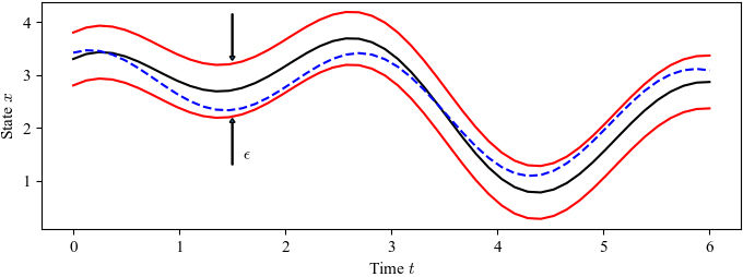
'''Figure 5.6:''' Illustration of Lyapunov’s concept of a stable solution. The solution represented by the solid line is stable if we can guarantee that all solutions remain within a tube of diameter ǫ by choosing initial conditions sufficiently close the solution. | '''Figure 5.6:''' Illustration of Lyapunov’s concept of a stable solution. The solution represented by the solid line is stable if we can guarantee that all solutions remain within a tube of diameter ǫ by choosing initial conditions sufficiently close the solution. | ||
| + | |||
| + | <nowiki> | ||
| + | # lyapunov_stability.py - illustration of Lyapunov stability | ||
| + | # RMM, 6 Apr 2024 | ||
| + | |||
| + | import matplotlib.pyplot as plt | ||
| + | import numpy as np | ||
| + | import control as ct | ||
| + | import fbs # FBS plotting customizations | ||
| + | |||
| + | t = np.linspace(0, 6) | ||
| + | x0 = np.sin(t) + 0.8 * np.cos(2.2 * t) + 2.5 | ||
| + | |||
| + | # Plot the centerline and bounds | ||
| + | fbs.figure('211') | ||
| + | plt.plot(t, x0, 'k') | ||
| + | plt.plot(t, x0 + 0.5, 'r', t, x0 - 0.5, 'r') | ||
| + | |||
| + | # Plot the signal | ||
| + | x = x0 - 0.4 * np.sin(t - 0.3) | ||
| + | plt.plot(t, x, 'b--') | ||
| + | |||
| + | # Label the axes | ||
| + | plt.xlabel("Time $t$") | ||
| + | plt.ylabel("State $x$") | ||
| + | |||
| + | # Add some arrows and label the range of stability | ||
| + | plt.arrow(1.5, 1.3, 0, 0.8, width=0.01, head_width=0.05) | ||
| + | plt.arrow(1.5, 4.15, 0, -0.8, width=0.01, head_width=0.05) | ||
| + | plt.text(1.6, 1.4, "$\\epsilon$") | ||
| + | |||
| + | fbs.savefig('figure-5.6-lyapunov_stability.png') | ||
| + | </nowiki> | ||
Latest revision as of 05:06, 7 April 2024
| Chapter | Dynamic Behavior |
|---|---|
| Figure number | 5.6 |
| Figure title | Illustration of Lyapunov’s concept of a stable solution |
| GitHub URL | https://github.com/murrayrm/fbs2e-python/blob/main/figure-5-6-lyapunov stability.py |
| Requires | python-control |
Figure 5.6: Illustration of Lyapunov’s concept of a stable solution. The solution represented by the solid line is stable if we can guarantee that all solutions remain within a tube of diameter ǫ by choosing initial conditions sufficiently close the solution.
# lyapunov_stability.py - illustration of Lyapunov stability
# RMM, 6 Apr 2024

import matplotlib.pyplot as plt
import numpy as np
import control as ct
import fbs                      # FBS plotting customizations

t = np.linspace(0, 6)
x0 = np.sin(t) + 0.8 * np.cos(2.2 * t) + 2.5

# Plot the centerline and bounds
fbs.figure('211')
plt.plot(t, x0, 'k')
plt.plot(t, x0 + 0.5, 'r', t, x0 - 0.5, 'r')

# Plot the signal
x = x0 - 0.4 * np.sin(t - 0.3)
plt.plot(t, x, 'b--')

# Label the axes
plt.xlabel("Time $t$")
plt.ylabel("State $x$")

# Add some arrows and label the range of stability
plt.arrow(1.5, 1.3, 0, 0.8, width=0.01, head_width=0.05)
plt.arrow(1.5, 4.15, 0, -0.8, width=0.01, head_width=0.05)
plt.text(1.6, 1.4, "$\\epsilon$")

fbs.savefig('figure-5.6-lyapunov_stability.png')
