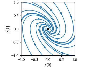
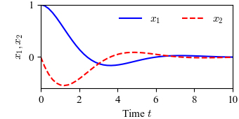
Figure 5.8: Phase portrait and time domain simulation for a system with a single asymptotically stable equilibrium point
Jump to navigation
Jump to search
| Chapter | Dynamic Behavior |
|---|---|
| Figure number | 5.8 |
| Figure title | Phase portrait and time domain simulation for a system with a single asymptotically stable equilibrium point |
| GitHub URL | https://github.com/murrayrm/fbs2e-python/blob/main/figure-5.8-asystable-eqpt.py |
| Requires | python-control |

|
|

|
Figure 5.7: Phase portrait and time domain simulation for a system with a single stable equilibrium point. The equilibrium point xe at the origin is stable since all trajectories that start near xe stay near xe.
# asystable_eqpt.py - plots for stable equlibrium point
# RMM, 7 Apr 2024

import matplotlib.pyplot as plt
import numpy as np
from math import pi
import control as ct
import control.phaseplot as pp
import fbs                      # FBS plotting customizations

m, b, k = 1, 1, 1
linsys = ct.ss([[0, 1], [-k/m, -b/m]], [[0], [1]], np.eye(2), 0)

# Draw the phase portrait
fbs.figure()
ct.phase_plane_plot(linsys, [-1, 1, -1, 1], 5)
plt.gca().set_aspect('equal')
plt.suptitle("")
fbs.savefig('figure-5.8.asystable_eqpt-pp.png')

fbs.figure('321')
plt.axis([0, 10, -0.5, 1])
timepts = np.linspace(0, 10)
response = ct.input_output_response(linsys, timepts, 0, [1, 0])
plt.plot(response.time, response.outputs[0], 'b', label="$x_1$")
plt.plot(response.time, response.outputs[1], 'r--', label="$x_2$")
plt.xlabel("Time $t$")
plt.ylabel("$x_1, x_2$")
plt.legend(loc='upper right', ncols=2, frameon=False)
fbs.savefig('figure-5.8-asystable_eqpt-time.png')
