Difference between revisions of "Figure 3.2: Illustration of a state model"
Jump to navigation
Jump to search
| Line 5: | Line 5: | ||
|GitHub URL=https://github.com/murrayrm/fbs2e-python/blob/main/figure-3.2-state_model.py | |GitHub URL=https://github.com/murrayrm/fbs2e-python/blob/main/figure-3.2-state_model.py | ||
}} | }} | ||
| − | [[Image:figure-3.2-state_model.png| | + | [[Image:figure-3.2-state_model.png|640px]] |
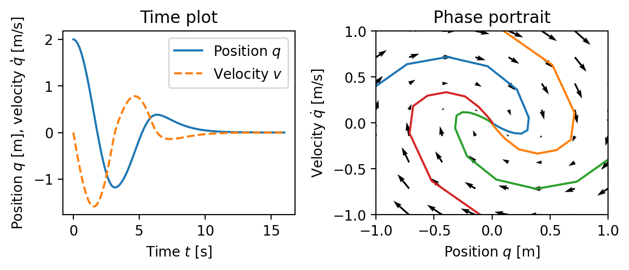
'''Figure 3.2''': Illustration of a state model. A state model gives the rate of change of the state as a function of the state. The plot on the left shows the evolution of the state as a function of time. The plot on the right, called a phase portrait, shows the evolution of the states relative to each other, with the velocity of the state denoted by arrows. | '''Figure 3.2''': Illustration of a state model. A state model gives the rate of change of the state as a function of the state. The plot on the left shows the evolution of the state as a function of time. The plot on the right, called a phase portrait, shows the evolution of the states relative to each other, with the velocity of the state denoted by arrows. | ||
Revision as of 00:57, 29 August 2021
| Chapter | System Modeling |
|---|---|
| Figure number | 3.2 |
| Figure title | Illustration of a state model |
| GitHub URL | https://github.com/murrayrm/fbs2e-python/blob/main/figure-3.2-state model.py |
| Requires | python-control |
Figure 3.2: Illustration of a state model. A state model gives the rate of change of the state as a function of the state. The plot on the left shows the evolution of the state as a function of time. The plot on the right, called a phase portrait, shows the evolution of the states relative to each other, with the velocity of the state denoted by arrows.
# figure-3.2-state_mode.py - illustration of a state model
# RMM, 2 Jul 2021
#
# Figure 3.2: Illustration of a state model. A state model gives the rate of
# change of the state as a function of the state. The plot on the left shows
# the evolution of the state as a function of time. The plot on the right,
# called a phase portrait, shows the evolution of the states relative to
# each other, with the velocity of the state denoted by arrows.
#

import numpy as np
import scipy as sp
import matplotlib.pyplot as plt
import control as ct

#
# Spring mass system with nonlinear dampling
#
# This function gives the dynamics for a dampled oscillator with nonlinear
# damping.  The states of the system are
#
#   x[0]        position
#   x[1]        velocity
#
# The nonlinear damping is implemented as a change in the linear damping
# coefficient at a small velocity.  This is intended to roughly correspond
# to some sort of stiction (and give an interesting phase portrait).  The
# default parameters for the system are given by
#
#   m = 1       mass, kg
#   k = 1       spring constant, N/m
#   b1 = 1      damping constant near origin, N-sec/m
#   b2 = 0.01   damping constant away from origin, N-sec/m
#   dth = 0.5   threshold for switching between damping
#
# This corresponds to a fairly lightly damped oscillator away from the origin.

def nlspringmass(x, t, u=0, m=1, k=1, b1=2, b2=0.01, dth=0.2):
    # Compute the friction force
    if abs(x[1]) < dth:
        Fb = b1 * x[1];
    elif x[1] < 0:
        Fb = -b1 * dth \
            + b2 * (x[1] + dth);
    else:
        Fb = b1 * dth \
            + b2 * (x[1] - dth);

    # Return the time derivative of the state
    return np.array([x[1], -k/m * x[0] - Fb/m])

#
# (a) Simulation of the nonlinear spring mass system
#
plt.subplot(2, 2, 1)

t = np.linspace(0, 16, 100)
y = sp.integrate.odeint(nlspringmass, [2, 0], t)

plt.plot(t, y[:, 0], '-', t, y[:, 1], '--')
plt.xlabel('Time $t$ [s]')
plt.ylabel('Position $q$ [m], velocity $\dot q$̇ [m/s]')
plt.title('Time plot')
plt.legend(['Position $q$', 'Velocity $v$'])

#
# (b) Generate a phase plot for the damped oscillator
#
plt.subplot(2, 2, 2)

ct.phase_plot(
    nlspringmass,               # dynamics
    (-1, 1, 8), (-1, 1, 8),     # X, Y range, npoints
    scale=0.2,
    X0=[[-1, 0.4], [0.1, 1], [1, -0.4], [-0.1, -1]])

plt.xlabel('Position $q$ [m]')
plt.ylabel('Velocity $\dot q$ [m/s]')
plt.title('Phase portrait')
plt.axis([-1, 1, -1, 1])

plt.tight_layout()
