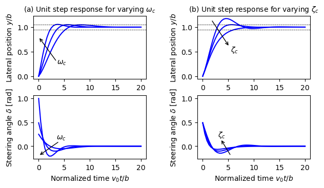
Figure 7.6: State feedback control of a steering system

Chapter	State Feedback
Figure number	7.6
Figure title	State feedback control of a steering system
GitHub URL	https://github.com/murrayrm/fbs2e-python/blob/main/example-7.4-steering place.py
Requires	python-control

Figure 7.6: State feedback control of a steering system. Unit step responses (from zero initial condition) obtained with controllers designed with $\zeta _{c}=0.7$ and $\omega _{c}=0.5$, $0.7$, and $1$ [rad/s] are shown in (a). The dashed lines indicate $\pm 5$% deviations from the setpoint. Notice that response speed increases with increasing $\omega _{c}$, but that large $\omega _{c}$ also give large initial control actions. Unit step responses obtained with a controller designed with $\omega _{c}=0.7$ and $\zeta _{c}=0.5$, $0.7$, and $1$ are shown in (b).

# example-7.4-steering_place.py - <Short description>
# RMM, 28 Nov 2024
#
# Figure 7.6: State feedback control of a steering system. Unit step
# responses (from zero initial condition) obtained with controllers
# designed with zeta_c = 0.7 and omega_c = 0.5, 0.7, and 1 [rad/s] are
# shown in (a). The dashed lines indicate ±5% deviations from the
# setpoint. Notice that response speed increases with increasing omega_c,
# but that large omega_c also give large initial control actions. Unit step
# responses obtained with a controller designed with omega_c = 0.7 and
# zeta_c = 0.5, 0.7, and 1 are shown 2in (b).

import control as ct
import numpy as np
import matplotlib.pyplot as plt
ct.use_fbs_defaults()

#
# System dynamics
#

# Get the normalized linear dynamics
from steering import linearize_lateral
sys = linearize_lateral(normalize=True, output_full_state=True)

# Function to place the poles at desired values
def steering_place(sys, omega, zeta):
    # Get the pole locations based on omega and zeta
    desired_poly = np.polynomial.Polynomial([omega**2, 2 * zeta * omega, 1])
    return ct.place(sys.A, sys.B, desired_poly.roots())

# Set up the plotting grid to match the layout in the book
fig = plt.figure(constrained_layout=True)
gs = fig.add_gridspec(3, 14)     # allow some space in the middle
left = slice(0, 6)
right = slice(7, 13)

#
# (a) Unit step response for varying omega_c
#

ax_pos = fig.add_subplot(gs[0, left])
ax_delta = fig.add_subplot(gs[1, left])
ax_pos.set_title(
    r"(a) Unit step response for varying $\omega_c$", size='medium')

timepts = np.linspace(0, 20)
zeta_c = 0.7
for omega_c in [0.5, 0.7, 1]:
    # Compute the gains for the controller
    K = steering_place(sys, omega_c, zeta_c)
    kf = omega_c**2

    # Compute the closed loop system
    clsys = ct.feedback(sys, K) * kf

    # Simulate the closed loop dynamics
    response = ct.forced_response(clsys, timepts, 1, X0=0)

    ax_pos.plot(response.time, response.states[0], 'b')
    ax_delta.plot(response.time, (kf - K @ response.states)[0], 'b')

# Label the plot
ax_pos.set_ylabel(r"Lateral position $y/b$")
ax_delta.set_xlabel(r"Normalized time $v_0 t/b$")
ax_delta.set_ylabel(r"Steering angle $\delta$ [rad]")

ax_pos.axhline(0.95, color='k', linestyle='--', linewidth=0.5)
ax_pos.axhline(1.05, color='k', linestyle='--', linewidth=0.5)
ax_pos.annotate(
    "", xy=(3.5, 0.3), xytext=[0, 0.8], arrowprops={'arrowstyle': '<-'})
ax_pos.text(3.6, 0.25, r"$\omega_c$")

ax_delta.annotate(
    "", xy=(4, 0.1), xytext=(0, -0.2), arrowprops={'arrowstyle': '<-'})
ax_delta.text(3.5, 0.15, r"$\omega_c$")

#
# (b) Unit step response for varying zeta_c
#

ax_pos = fig.add_subplot(gs[0, right], sharey=ax_pos)
ax_delta = fig.add_subplot(gs[1, right], sharey=ax_delta)
ax_pos.set_title(
    r"(b) Unit step response for varying $\zeta_c$", size='medium')

timepts = np.linspace(0, 20)
omega_c = 0.7
for zeta_c in [0.5, 0.7, 1]:
    # Compute the gains for the controller
    K = steering_place(sys, omega_c, zeta_c)
    kf = omega_c**2

    # Compute the closed loop system
    clsys = ct.feedback(sys, K) * kf

    # Simulate the closed loop dynamics
    response = ct.forced_response(clsys, timepts, 1, X0=0)

    ax_pos.plot(response.time, response.states[0], 'b')
    ax_delta.plot(response.time, (kf - K @ response.states)[0], 'b')

# Label the plot
ax_pos.set_ylabel(r"Lateral position $y/b$")
ax_delta.set_xlabel(r"Normalized time $v_0 t/b$")
ax_delta.set_ylabel(r"Steering angle $\delta$ [rad]")

ax_pos.axhline(0.95, color='k', linestyle='--', linewidth=0.5)
ax_pos.axhline(1.05, color='k', linestyle='--', linewidth=0.5)
ax_pos.annotate(
    "", xy=(1.7, 1.15), xytext=(5.2, 0.6), arrowprops={'arrowstyle': '<-'})
ax_pos.text(5.5, 0.5, r"$\zeta_c$")

ax_delta.annotate(
    "", xy=(5.5, -0.2), xytext=(3.5, 0.15), arrowprops={'arrowstyle': '<-'})
ax_delta.text(3, 0.2, r"$\zeta_c$")

# Save the figure
fig.align_ylabels()
plt.savefig("figure-7.4-steering_place.png", bbox_inches='tight')