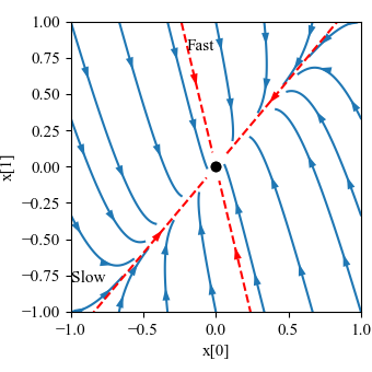
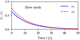
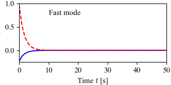
Figure 6.5: Modes for a second-order system with real eigenvalues

Chapter	Linear Systems
Figure number	6.5
Figure title	The notion of modes for a second-order system with real eigenvalues.
GitHub URL	https://github.com/murrayrm/fbs2e-python/blob/main/figure-6.5-modes.py
Requires	python-control, springmass.py

Figure 6.5: The notion of modes for a second-order system with real eigenvalues. The left figure shows the phase portrait and the modes corresponding to solutions that start on the eigenvectors (bold lines). The corresponding time functions are shown on the right.

# superposition.py - superposition of homogeneous and particular solutions
# RMM, 19 Apr 2024

import matplotlib.pyplot as plt
import numpy as np
import control as ct
import fbs                      # FBS plotting customizations

# Spring mass system
from springmass import springmass       # use spring mass dynamics
sys = springmass / springmass(0).real   # normalize the response to 1
X0 = [2, -1]                            # initial condition

# Create input vectors
tvec = np.linspace(0, 60, 100)
u1 = 0 * tvec
u2 = np.hstack([tvec[0:50]/tvec[50], 1 - tvec[0:50]/tvec[50]])

# Run simulations for the different cases
homogeneous = ct.forced_response(sys, tvec, u1, X0=X0)
particular = ct.forced_response(sys, tvec, u2)
complete = ct.forced_response(sys, tvec, u1 + u2, X0=X0)

# Plot results
fig, axs = plt.subplots(3, 3, figsize=[8, 4], layout='tight')
for i, resp in enumerate([homogeneous, particular, complete]):
    axs[i, 0].plot(resp.time, resp.inputs)
    axs[0, 0].set_title("Input $u$")
    axs[i, 0].set_ylim(-2, 2)
    
    axs[i, 1].plot(
        resp.time, resp.states[0], 'b',
        resp.time, resp.states[1], 'r--')
    axs[0, 1].set_title("States $x_1$, $x_2$")
    axs[i, 1].set_ylim(-2, 2)

    axs[i, 2].plot(resp.time, resp.outputs)
    axs[0, 2].set_title("Output $y$")
    axs[i, 2].set_ylim(-2, 2)

# Label the plots
axs[0, 0].set_ylabel("Homogeneous")
axs[1, 0].set_ylabel("Particular")
axs[2, 0].set_ylabel("Complete")
for i in range(3):
    axs[2, i].set_xlabel("Time $t$ [s]")

# Save the figure
fbs.savefig('figure-6.1-superposition.png')