Figure 4.12: Internet congestion control
Jump to navigation
Jump to search
| Chapter | Examples |
|---|---|
| Figure number | 4.12 |
| Figure title | Internet congestion control |
| GitHub URL | https://github.com/murrayrm/fbs2e-python/blob/main/figure-4.12-congctrl eqplot.py |
| Requires | python-control |
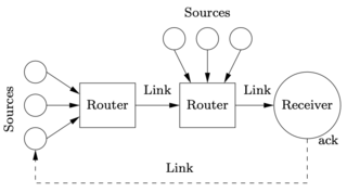
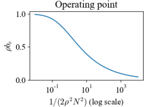
Figure 4.12: Internet congestion control. (a) Source computers send information to routers, which forward the information to other routers that eventually connect to the receiving computer. When a packet is received, an acknowledgment packet is sent back through the routers (not shown). The routers buffer information received from the sources and send the data across the outgoing link. (b) The equilibrium buffer size be for a set of N identical computers sending packets through a single router with drop probability ρb.
# congctrl_eqplot.py - congestion control equilibrium point plot
# RMM, 29 Jun 2007 (converted from MATLAB)
#
# The equilibrium buffer size be for a set of N identical computers sending
# packets through a single router with drop probability ρb.
#

import matplotlib.pyplot as plt
import numpy as np
import scipy.optimize

# Range of values to plot (\alpha = 1/(2\rho^2 N^2)
alpha_vals = np.logspace(-2, 4)

# Solve for the equilibrium value of \rho b_e
bratio_vals = []
for alpha in alpha_vals:
    # Define a function for the equilibrium point (equation (4.22))
    def equilibrium(bratio):
        return alpha * bratio**3 + bratio - 1

    bratio = scipy.optimize.fsolve(equilibrium, 0)
    bratio_vals.append(bratio)

# Plot the equilibrium buffer length
plt.semilogx(alpha_vals, bratio_vals)
plt.xlabel(r"$1/(2 \rho^2 N^2)$ (log scale)")
plt.ylabel(r"$\rho b_{e}$")
plt.title("Operating point")

