Difference between revisions of "Figure 5.4: Equilibrium points for an inverted pendulum"
Jump to navigation
Jump to search
(Created page with "{{Figure |Chapter=Dynamic Bevier |Figure number=5.4 |Sort key=504 |Figure title=Equilibrium points for an inverted pendulum |GitHub URL=https://github.com/murrayrm/fbs2e-pytho...") |
|||
| Line 1: | Line 1: | ||
{{Figure | {{Figure | ||
| − | |Chapter=Dynamic | + | |Chapter=Dynamic Behavior |
|Figure number=5.4 | |Figure number=5.4 | ||
|Sort key=504 | |Sort key=504 | ||
Latest revision as of 16:22, 7 April 2024
| Chapter | Dynamic Behavior |
|---|---|
| Figure number | 5.4 |
| Figure title | Equilibrium points for an inverted pendulum |
| GitHub URL | https://github.com/murrayrm/fbs2e-python/blob/main/figure-5.4-invpend phaseplot.py |
| Requires | python-control |
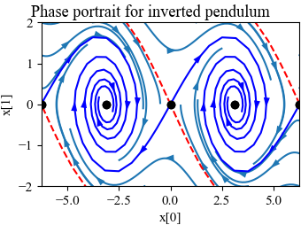
Figure 5.4: Equilibrium points for an inverted pendulum. An inverted pendulum is a model for a class of balance systems in which we wish to keep a system upright, such as a rocket (a). Using a simplified model of an inverted pendulum (b), we can develop a phase portrait that shows the dynamics of the system (c). The system has multiple equilibrium points, marked by the solid dots along the x2 = 0 line.
# invepend_phaseplot.py - inverted pendulum phase plots
# RMM, 6 Apr 2024

import matplotlib.pyplot as plt
import numpy as np
from math import pi
import control as ct
import control.phaseplot as pp
import fbs                      # FBS plotting customizations

def invpend_update(t, x, u, params):
    m, l, b, g = params['m'], params['l'], params['b'], params['g']
    return [x[1], -b/m * x[1] + (g * l / m) * np.sin(x[0])]
invpend = ct.nlsys(
    invpend_update, states=2, inputs=0, name='inverted pendulum',
    params={'m': 1, 'l': 1, 'b': 0.2, 'g': 1})

fbs.figure()
ct.phase_plane_plot(
    invpend, [-2*pi, 2*pi, -2, 2], 4, gridspec=[6, 6],
    plot_separatrices={'timedata': 20, 'arrows': 4})
fbs.savefig('figure-5.4-invpend_phaseplotf.png')
