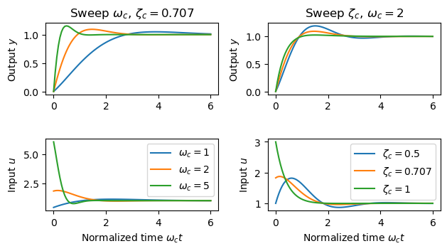
Figure 2.9: Responses to a unit step change in the reference signal for different values of the design parameters

Chapter	Feedback Principles
Figure number	2.9
Figure title	Responses to a unit step change in the reference signal for different values of the design parameters
GitHub URL	https://github.com/murrayrm/fbs2e-python/blob/main/figure-2.9-secord stepresp.py
Requires	python-control

Figure 2.9: Responses to a unit step change in the reference signal for different values of the design parameters $\omega _{\text{c}}$ and $\zeta _{\text{c}}$. The left figure shows responses for fixed $\zeta _{\text{c}}=$0.707 and $\omega _{\text{c}}=$ 1, 2, and 5. The right figure shows responses for $\omega _{\text{c}}=$ 2 and $\zeta _{\text{c = }}$ 0.5, 0.707, and 1. The process parameters are $a=b=1$. The initial value of the control signal is $k_{\text{p}}$.

# figure-2.9-secord_stepresp.py - step responses for second order systems
# RMM, 21 Jun 2021
#
# Responses to a unit step change in the reference signal for different
# values of the design parameters \omega_c and \zeta_c. The left column
# shows responses for fixed \zeta_c = 0.707 and \omega_c = 1, 2, and 5. The
# right figure column responses for \omega_c = 2 and \zeta_c = 0.5, 0.707,
# and 1. The process parameters are a = b = 1. The initial value of the
# control signal is kp.
#

import numpy as np
import matplotlib.pyplot as plt
import control as ct

# Process model
b = 1; a = 1
P = ct.tf([b], [1, a])

# Set the simulation time vector
time = np.linspace(0, 6, 100)

#
# Omega sweep
#

# Choose gains to use
wc_list = [1, 2, 5]
zc = 0.707

for wc in wc_list:
    kp = (2 * zc * wc - a) / b
    ki = wc**2
    C = ct.tf([kp, ki], [1, 0])
    
    Gyr = P*C / (1 + P*C)
    Gur = C / (1 + P*C)

    t, y = ct.step_response(Gyr, time)
    t, u = ct.step_response(Gur, time)

    if 'w_y_ax' not in locals():
        w_y_ax = plt.subplot(3, 2, 1)
        plt.ylabel('Output $y$')
        plt.title("Sweep $\omega_c$, $\zeta_c = %g$" % zc)
    w_y_ax.plot(t, y)

    if 'w_u_ax' not in locals():
        w_u_ax = plt.subplot(3, 2, 3)
        plt.ylabel('Input $u$')
        plt.xlabel('Normalized time $\omega_c t$')
    w_u_ax.plot(t, u, label="$\omega_c = %g$" % wc)

# Label the omega sweep curves
w_u_ax.legend(loc="upper right")

#
# Zeta sweep
#

# Figure out frequency of critical damping
wc = 2
zc_list = [0.5, 0.707, 1]

# Plot results for different resonate frequencies
for zc in zc_list:
    kp = (2 * zc * wc - a) / b
    ki = wc**2
    C = ct.tf([kp, ki], [1, 0])
    
    Gyr = P*C / (1 + P*C)
    Gur = C / (1 + P*C)

    t, y = ct.step_response(Gyr, time)
    t, u = ct.step_response(Gur, time)

    if 'z_y_ax' not in locals():
        z_y_ax = plt.subplot(3, 2, 2)
        plt.ylabel('Output $y$')
        plt.title("Sweep $\zeta_c$, $\omega_c = %g$" % wc)
    z_y_ax.plot(t, y)

    if 'z_u_ax' not in locals():
        z_u_ax = plt.subplot(3, 2, 4)
        plt.ylabel('Input $u$')
        plt.xlabel('Normalized time $\omega_c t$')
    z_u_ax.plot(t, u, label="$\zeta_c = %g$" % zc)

# Label the zeta sweep curves
z_u_ax.legend(loc="upper right")

# Overalll figure labeling
plt.tight_layout()