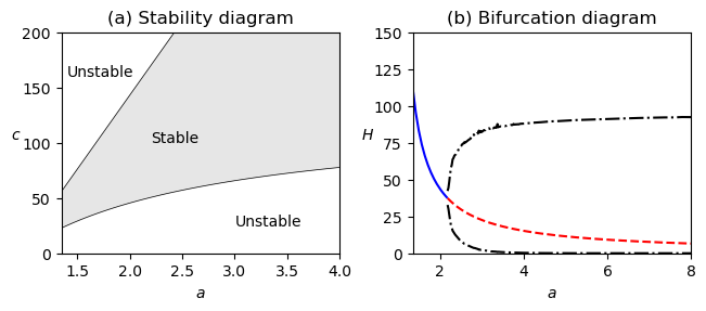
Figure 5.18: Bifurcation analysis of the predator–prey system

Chapter	Dynamic Behavior
Figure number	5.18
Figure title	Bifurcation analysis of the predator-prey system
GitHub URL	https://github.com/murrayrm/fbs2e-python/blob/main/example-5.16-predprey bif.py
Requires	python-control, predprey.py

Figure 5.18': Bifurcation analysis of the predator–prey system. (a) Parametric stability diagram showing the regions in parameter space for which the system is stable. (b) Bifurcation diagram showing the location and stability of the equilibrium point as a function of $a$. The solid line represents a stable equilibrium point, and the dashed line represents an unstable equilibrium point. The dash-dotted lines indicate the upper and lower bounds for the limit cycle at that parameter value (computed via simulation). The nominal values of the parameters in the model are $a=3.2$, $b=0.6$, $c=50$, $d=0.56$, $k=125$, and $r=1.6$.

# example-5.16-predprey_bif.py - predator-prey stability analysis
# RMM, 18 Nov 2024
#
# Figure 5.18: Bifurcation analysis of the predator–prey system. (a)
# Parametric stability diagram showing the regions in parameter space for
# which the system is stable. (b) Bifurcation diagram showing the location
# and stability of the equilib- rium point as a function of a. The solid
# line represents a stable equilibrium point, and the dashed line
# represents an unstable equilibrium point. The dash-dotted lines indicate
# the upper and lower bounds for the limit cycle at that parameter value
# (computed via simulation). The nominal values of the parameters in the
# model are a = 3.2, b = 0.6, c = 50, d = 0.56, k = 125, and r = 1.6.

import control as ct
import numpy as np
import scipy
import matplotlib.pyplot as plt
ct.use_fbs_defaults()

#
# System dynamics
#

from predprey import predprey, predprey_params

# Create a function to compute the real part of the largest eigenvalue
def maxeig(a, c):
    # Initialize parameter values
    r, d, b, k = map(predprey_params.get, ['r', 'd', 'b', 'k'])
    params = {'a': a, 'c': c}
    
    # Equilibrium point from equations (4.33) and (4.34)
    xeq = [(c*d) / (a*b - d), (b*c*r)*(a*b*k - c*d - d*k)/(k * (a*b - d)**2)]

    # Linearization
    A = ct.linearize(predprey, xeq, 0, params=params).A
    
    return np.max(np.linalg.eig(A).eigenvalues.real)

# Set up the plotting grid to match the layout in the book
fig = plt.figure(constrained_layout=True)
gs = fig.add_gridspec(2, 2)

#
# (a) Stability diagram
#
# To find the boundaries of stability in terms of the parameters $a$ and
# $c$, we scan over the $a$ parameter and find the values of $c$ that cause
# the real part of one of the eigenvalues to be zero.
#

ax = fig.add_subplot(gs[0, 0])  # first row, first column
ax.set_title("(a) Stability diagram")

avals = np.linspace(1.3, 4, 50)
cvals_lower, cvals_upper = [], []
last_lower, last_upper = 5, 100
for a in avals:
    sol1 = scipy.optimize.root(
        lambda c: maxeig(a, c), last_lower, method='broyden1')
    if sol1.success:
        last_lower = sol1.x.item()
        cvals_lower.append(last_lower)
    else:
        print(sol1.message)
        cvals_lower.append(np.nan)
    
    sol2 = scipy.optimize.root(lambda c: maxeig(a, c), last_upper)
    if sol2.success:
        last_upper = sol2.x.item()
        cvals_upper.append(last_upper)
    else:
        cvals_upper.append(np.nan)

ax.plot(avals, cvals_lower, 'k', linewidth=0.5)
ax.plot(avals, cvals_upper, 'k', linewidth=0.5)
ax.fill_between(avals, cvals_lower, cvals_upper, color='0.9')

ax.set_xlabel("$a$")
ax.set_ylabel("$c$", rotation=0)
ax.text(1.4, 160, "Unstable")
ax.text(2.2, 100, "Stable")
ax.text(3, 25, "Unstable")
ax.axis('tight')
ax.axis([1.35, 4, 0, 200])

#
# (b) Bifurcation diagram
#

ax = fig.add_subplot(gs[0, 1])  # first row, second column
ax.set_title("(b) Bifurcation diagram")

# Create lists to hold the values of the different branches on the plot
stable_H, unstable_H = [], []   # Equilibrium point
lower_H, upper_H = [], []       # Limit cycle bounds

# Set the values of 'a' to be denser near the bifurcation point
avals = np.hstack(
    [np.linspace(1.35, 2, 10), np.linspace(2, 4, 100), np.linspace(4, 8, 20)])

# Set up the remaining parameters for the simulation
timepts = np.linspace(0, 300, 5000)
params = predprey_params

# Compute the branches of the bifurcation diagram 
for a in avals:
    # Set the parameter values
    params['a'] = a

    # Equilibrium point from equations (4.33) and (4.34)
    r, d, b, k, c = map(predprey_params.get, ['r', 'd', 'b', 'k', 'c'])
    xeq = [(c*d) / (a*b - d), (b*c*r)*(a*b*k - c*d - d*k)/(k * (a*b - d)**2)]

    # Check stability
    if maxeig(a, params['c']) < 0:
        # Stable branch
        stable_H.append(xeq[0])
        [vlist.append(np.nan) for vlist in [unstable_H, lower_H, upper_H]]
    else:
        # Unstable branch
        unstable_H.append(xeq[0])
        stable_H.append(np.nan)

        # Run a simulation to figure out size of the limit cycle
        resp = ct.input_output_response(
            predprey, timepts, X0=np.array(xeq) + 0.1, params=params)
        lower_H.append(np.min(resp.outputs[0, -500:]))
        upper_H.append(np.max(resp.outputs[0, -500:]))

# Plot the different branches
ax.plot(avals, stable_H, 'b-')
ax.plot(avals, unstable_H, 'r--')
ax.plot(avals, lower_H, 'k-.')
ax.plot(avals, upper_H, 'k-.')

# Label the plot
ax.set_xlabel("$a$")
ax.set_ylabel("$H$", rotation=0)
ax.axis('tight')
ax.axis([1.35, 8, 0, 150])

# Save the figure
plt.savefig("figure-5.18-predprey_bif.png", bbox_inches='tight')