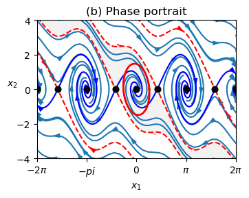
Figure 5.17: Stabilized inverted pendulum

Chapter	Dynamic Behavior
Figure number	5.17
Figure title	Stabilized inverted pendulum
GitHub URL	https://github.com/murrayrm/fbs2e-python/blob/main/example-5.14-invpend stabilized.py
Requires	python-control

Figure 5.17: Stabilized inverted pendulum. A control law applies a force u at the bottom of the pendulum to stabilize the inverted position (a) [not shown]. The phase portrait (b) shows that the equilibrium point corresponding to the vertical position is stabilized. The shaded region indicates the set of initial conditions that converge to the origin. The ellipse corresponds to a level set of a Lyapunov function $V(x)$ for which $V(x)>0$ and ${\dot {V}}(x)<0$ for all points inside the ellipse. This can be used as an estimate of the region of attraction of the equilibrium point. The actual dynamics of the system evolve on a manifold (c) [not shown].

# example-5.14-invpend_stabilized.py - stabilized inverted pendulum
# RMM, 17 Nov 2024

# Figure 5.17: Stabilized inverted pendulum. A control law applies a
# force u at the bottom of the pendulum to stabilize the inverted
# position (a). The phase portrait (b) shows that the equilibrium
# point corresponding to the vertical position is stabilized. The
# shaded region indicates the set of initial conditions that converge
# to the origin. The ellipse corresponds to a level set of a Lyapunov
# function V (x) for which V (x) > 0 and V ̇ (x) < 0 for all points
# inside the ellipse. This can be used as an estimate of the region of
# attraction of the equilibrium point. The actual dynamics of the
# system evolve on a manifold (c).

import control as ct
import numpy as np
import matplotlib.pyplot as plt
from math import pi, sin, cos, sqrt
ct.use_fbs_defaults()

#
# System dynamics
#

# Stablized (and normalized) inverted pendulum dynamics
def balpend_update(t, x, v, params):
    a = params.get('a', 2)
    u = -2 * a * sin(x[0]) - x[1] * cos(x[0])
    return [x[1], sin(x[0]) + u * cos(x[0])]
balpend = ct.nlsys(
    balpend_update, states=2, inputs=0, name='inverted pendulum')


# Set up the plotting grid to match the layout in the book
fig = plt.figure(constrained_layout=True)
gs = fig.add_gridspec(2, 4)
ax = fig.add_subplot(gs[0, 1:3])

# Generate the phase plot (easy part)
cplt = ct.phase_plane_plot(
    balpend, [-2*pi, 2*pi, -4, 4], 4.5, gridspec=[10, 10],
    plot_separatrices={'timedata': np.linspace(0, 20, 500), 'arrows': 1},
    ax=ax)

#
# Next we need to shade the region of attraction containing the origin.  We
# do this by extracting out the bounding separatrices and then filling in
# the region between them, using some messy NumPy/Matplotlib commands...
#

# Get the separatrices on either side of the origin
for line in cplt.lines[0]:
    xdata, ydata = line.get_data()
    if line.get_linestyle() != '--' or abs(ydata[-1]) > 0.1:
        continue                # Not the line we are looking for

    # Extract out the separatrices for the middle region
    if xdata[-1] < 0 and xdata[-1] > -2 and ydata[-1] > 0:
        ul = (xdata[::-1], ydata[::-1])         # Sort along increasing y
    elif xdata[-1] < 0 and xdata[-1] > -2 and ydata[-1] < 0:
        ll = (xdata, ydata)
    elif xdata[-1] > 0 and xdata[-1] < 2 and ydata[-1] > 0:
        ur = (xdata[::-1], ydata[::-1])         # Sort along increasing y
    elif xdata[-1] > 0 and xdata[-1] < 2 and ydata[-1] < 0:
        lr = (xdata, ydata)

# Shade the region between the separatrices (including the middle)
ax.fill_betweenx(ul[1], ul[0], np.interp(ul[1], ur[1], ur[0]), color='0.95')
ax.fill_betweenx(lr[1], np.interp(lr[1], ll[1], ll[0]), lr[0], color='0.95')
ax.fill_betweenx(
    [ul[1][0], ll[1][-1]], [ul[0][0], ll[0][-1]], [ur[0][0], lr[0][-1]],
    color='0.95')

# Add the Lypaunov level set
A = balpend.linearize(0, 0).A   # Linearized dynamics matrix
P = ct.lyap(A.T, np.eye(2))     # Solve Lyapunov equation for P

# Figure out the states along the level set
rho = 1.2                       # value of the level set
xval, yval = [], []
for theta in np.linspace(0, 2*pi, 100):
    # Find the length of state vector at this angle that gives V(x) = 1
    r = 1 / sqrt(np.array([cos(theta), sin(theta)]).T @ P @ 
                 np.array([cos(theta), sin(theta)]))
    xval.append(rho * r * cos(theta))
    yval.append(rho * r * sin(theta))
ax.plot(xval, yval, 'r-', linewidth=2)

# Label the plot
ax.set_xticks([-2*pi, -pi, 0, pi, 2*pi])
ax.set_xticklabels([r'$-2\pi$', r'$-pi$', r'$0$', r'$\pi$', r'$2\pi$'])
ax.set_xlabel('$x_1$')
ax.set_ylabel('$x_2$', rotation=0)
ax.set_title("(b) Phase portrait")

plt.savefig('figure-5.17-balpend_phaseplot.png', bbox_inches='tight')