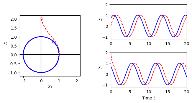
Figure 5.13: Solution curves for a stable limit cycle

Chapter	Dynamic Behavior
Figure number	5.13
Figure title	Solution curves for a stable limit cycle
GitHub URL	https://github.com/murrayrm/fbs2e-python/blob/main/example-5.9-limit cycle stability.py
Requires	python-control

Figure 5.12: Solution curves for a stable limit cycle. The phase portrait on the left shows that the trajectory for the system rapidly converges to the stable limit cycle. The starting points for the trajectories are marked by circles in the phase portrait. The time domain plots on the right show that the states do not converge to the solution but instead maintain a constant phase error.

# example-5.9-limit_cycle_stability.py - Solution curves for stable limit cycle
# RMM, 16 Nov 2024 (with initial converstion from MATLAB by ChatGPT)
#
# Figure 5.13: Solution curves for a stable limit cycle. The phase portrait
# on the left shows that the trajectory for the system rapidly converges to
# the stable limit cycle. The starting points for the trajectories are
# marked by circles in the phase portrait. The time domain plots on the
# right show that the states do not converge to the solution but instead
# maintain a constant phase error.

import control as ct
import numpy as np
import matplotlib.pyplot as plt
from scipy.integrate import solve_ivp
ct.use_fbs_defaults()

#
# System dynamics
#

def limcyc(t, x):
    E = x[0]**2 + x[1]**2
    xdot1 = x[1] + x[0] * (1 - E)
    xdot2 = -x[0] + x[1] * (1 - E)
    return [xdot1, xdot2]

# Set up the plotting grid to match the layout in the book
fig = plt.figure(constrained_layout=True)
gs = fig.add_gridspec(8, 10)

# Simulation settings
ts = 20
tspan = (0, ts)
x01 = [0, 2]
x02 = [1/np.sqrt(2), 1/np.sqrt(2)]

#
# (a) Phase plane plot
#

ax = fig.add_subplot(gs[1:5, :4])      # left plot

# Solve the differential equations
sol1 = solve_ivp(limcyc, tspan, x01, t_eval=np.linspace(*tspan, 1000))
sol2 = solve_ivp(limcyc, tspan, x02, t_eval=np.linspace(*tspan, 1000))

# Plot phase plane
ax.plot(sol1.y[0], sol1.y[1], 'r--')
ax.plot(sol2.y[0], sol2.y[1], 'b-')
ax.scatter(0, 2, facecolors='none', edgecolors='r')
ax.scatter(1/np.sqrt(2), 1/np.sqrt(2), facecolors='none', edgecolors='b')

ax.axhline(0, color='k')
ax.axvline(0, color='k')
ax.axis('square')
ax.axis([-1.2, 2.2, -1.2, 2.2])
ax.set_xlabel('$x_1$')
ax.set_ylabel('$x_2$', rotation=0)

#
# (b) Time traces
#

ax = fig.add_subplot(gs[1:3, 5:])      # upper right plot
ax.plot(sol1.t, sol1.y[0], 'r--')
ax.plot(sol2.t, sol2.y[0], 'b-')
ax.set_xlim([0, 20])
ax.set_ylim([-1.2, 2])
ax.set_ylabel('$x_1$', rotation=0)

ax = fig.add_subplot(gs[3:5, 5:])      # upper right plot
ax.plot(sol1.t, sol1.y[1], 'r--')
ax.plot(sol2.t, sol2.y[1], 'b-')
ax.set_xlim([0, 20])
ax.set_ylim([-1.2, 2])
ax.set_ylabel('$x_2$', rotation=0)
ax.set_xlabel('Time $t$')

plt.savefig('figure-5.13-limit_cycle_stability.png', bbox_inches='tight')