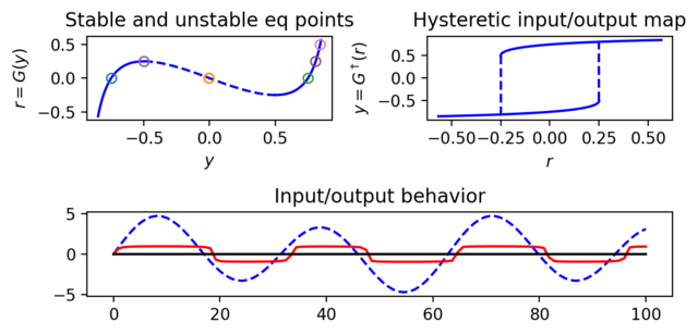
Figure 2.19: System with positive feedback and saturation

Chapter	Feedback Principles
Figure number	2.19
Figure title	System with positive feedback and saturation
GitHub URL	https://github.com/murrayrm/fbs2e-python/blob/main/figure-2.19-posfbk saturation.py
Requires	python-control

Figure 2.19: System with positive feedback and saturation. (a) For a # fixed reference value r, the intersections with the curve $r=G(y)$ corresponds to equilibrium points for the system. Equilibrium points at selected values of r are shown by circles (note that for some reference values there are multiple equilibrium points). Arrows indicate the sign of the derivative of $y$ away from the equilibrium points, with the solid portions of $r=G(y)$ representing stable equilibrium points and dashed portions representing unstable equilibrium points. (b) The hysteretic input/output map given by $y=G+(r)$, showing that some values of $r$ have single equilibrium points while others have two possible (stable) steady-state output values. (c) Simulation of the system dynamics showing the reference $r$ (dashed curve) and the output y (solid curve).

# figure-2.19-posfbk_saturation.py - positive feedback with saturation
# RMM, 22 Jun 2021
#
# Figure 2.19: System with positive feedback and saturation. (a) For a
# fixed reference value r, the intersections with the curve r = G(y)
# corresponds to equilibrium points for the system. Equilibrium points
# at selected values of r are shown by circles (note that for some
# reference values there are multiple equilibrium points). Arrows
# indicate the sign of the derivative of y away from the equilibrium
# points, with the solid portions of r = G(y) representing stable
# equilibrium points and dashed portions representing unstable
# equilibrium points. (b) The hysteretic input/output map given by y =
# G+(r), showing that some values of r have single equilibrium points
# while others have two possible (stable) steady-state output val-
# ues. (c) Simulation of the system dynamics showing the reference r
# (dashed curve) and the output y (solid curve).

import numpy as np
import matplotlib.pyplot as plt
import control as ct

# Nonlinearity: forward and reverse
def F(x):
    return x / (1 + np.abs(x))

def Finv(y):
    return y / (1 - np.abs(y))

# Equilibrium calculation
a = 1; b = 4;                   # parameters for the system dynamics
def G(y, a=a, b=b):
    return a * Finv(y) / b - y

#
# Stable and unstable equilibrium points
#
plt.subplot(2, 2, 1)
plt.title('Stable and unstable eq points')
plt.xlabel('$y$')
plt.ylabel('$r = G(y)$')

# Define the stable and unstable branches
ymax = -1 + np.sqrt(a/b)        # First maximum (negative value)
y_stable = np.linspace(-ymax, 0.85, 100)
y_unstable = np.linspace(ymax, -ymax, 100)

# Plot the locus of equilibrium piots
plt.plot(-y_stable, G(-y_stable), 'b-')
plt.plot(y_unstable, G(y_unstable), 'b--')
plt.plot(y_stable, G(y_stable), 'b-')

# Plot individual equlibrium points
for r in [0, G(ymax), 0.5]:
    # Find the values intersecting this value of r
    y_left_arg = np.argwhere(G(-y_stable) >= r)
    if y_left_arg.size > 0:
        y = -y_stable[y_left_arg[-1].item()]
        plt.plot(y, r, 'o', fillstyle='none')

    y_center_arg = np.argwhere(G(y_unstable) >= r)
    if y_center_arg.size > 0:
        y = y_unstable[y_center_arg[-1].item()]
        plt.plot(y, r, 'o', fillstyle='none')

    y_right_arg = np.argwhere(G(y_stable) <= r)
    if y_right_arg.size > 0:
        y = y_stable[y_right_arg[-1].item()]
        plt.plot(y, r, 'o', fillstyle='none')
        
#
# Hysteretic input/output map y=G+(r)
#
plt.subplot(2, 2, 2)
plt.title('Hysteretic input/output map')
plt.xlabel('$r$')
plt.ylabel(r'$y = G^\dagger(r)$')

# Plot y versus r (multi-valued)
plt.plot(G(y_stable), y_stable, 'b-')       # Upper branch
plt.plot(G(-y_stable), -y_stable, 'b-')     # Lower branch

# Transition lines (look for intersection on opposite branch)
plt.plot(
    [G(y_stable[0]), G(y_stable[0])],
    [y_stable[0],
     -y_stable[np.argwhere(G(-y_stable) > G(y_stable[0]))[-1].item()]],
    'b--')
plt.plot(
    [G(-y_stable[0]), G(-y_stable[0])],
    [-y_stable[0],
     y_stable[np.argwhere(G(y_stable) < G(-y_stable[0]))[-1].item()]],
    'b--')

#
# Input/output behavior
#
plt.subplot(2, 1, 2)
plt.title('Input/output behavior')

# Closed loop dynamics
linsys = ct.tf([b], [1, a])
nonlin = ct.nlsys(
    updfcn=None, outfcn=lambda t, x, u, params: F(u),
    inputs=1, outputs=1)
posfbk = ct.feedback(nonlin * linsys, 1, 1)

# Simulate and plot
t = np.linspace(0, 100, 100)
r = 4 * np.sin(0.2 * t) + np.sin(0.1 * t)
t, y = ct.input_output_response(posfbk, t, r)
plt.plot(t, r, 'b--')
plt.plot(t, y, 'r')
plt.plot(t, np.zeros_like(t), 'k')

plt.tight_layout()