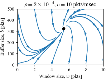
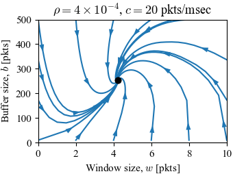
Figure 5.10: Phase portraits for a congestion control protocol running with N = 60 identical source computers

Chapter	Dynamic Behavior
Figure number	5.10
Figure title	Phase portraits for a congestion control protocol running with N = 60 identical source computers.
GitHub URL	https://github.com/murrayrm/fbs2e-python/blob/main/figure-5.10-congctrl dynamics.py
Requires	python-control

 

Figure 5.10: Phase portraits for a congestion control protocol running with $N=60$ identical source computers. The equilibrium values correspond to a fixed window at the source, which results in a steady-state buffer size and corresponding transmission rate. A faster link (b) uses a smaller buffer size since it can handle packets at a higher rate.

# congctrl-dynamics.py - phase plots for congestion control dynamis
# RMM, 7 Apr 2024

import matplotlib.pyplot as plt
import numpy as np
import control as ct
import fbs                      # FBS plotting customizations

# Define the system dynamics
def _congctrl_update(t, x, u, params):
    # Number of sources per state of the simulation
    M = x.size - 1                      # general case
    assert M == 1                       # make sure nothing funny happens here

    # Remaining parameters
    N = params.get('N', M)              # number of sources
    rho = params.get('rho', 2e-4)       # RED parameter = pbar / (bupper-blower)
    c = params.get('c', 10)             # link capacity (Mp/ms)

    # Compute the derivative (last state = bdot)
    return np.append(
        c / x[M] - (rho * c) * (1 + (x[:-1]**2) / 2),
        N/M * np.sum(x[:-1]) * c / x[M] - c)

congctrl = ct.nlsys(
    _congctrl_update, states=2, inputs=0,
    params={'N': 60, 'rho': 2e-4, 'c': 10})

fbs.figure()
ct.phase_plane_plot(congctrl, [0, 10, 10, 500], 100)
plt.axis([0, 10, 0, 500])
plt.suptitle("")
plt.title("$\\rho = 2 \\times 10^{-4}$, $c = 10$ pkts/msec")
plt.xlabel("Window size, $w$ [pkts]")
plt.ylabel("Buffer size, $b$ [pkts]")
fbs.savefig('figure-5.10-congctrl_dynamics-pp1.png')

fbs.figure()
ct.phase_plane_plot(
    congctrl, [0, 10, 10, 500], 100,
    params={'rho': 4e-4, 'c': 20})
plt.axis([0, 10, 0, 500])
plt.suptitle("")
plt.title("$\\rho = 4 \\times 10^{-4}$, $c = 20$ pkts/msec")
plt.xlabel("Window size, $w$ [pkts]")
plt.ylabel("Buffer size, $b$ [pkts]")
fbs.savefig('figure-5.10-congctrl_dynamics-pp2.png')