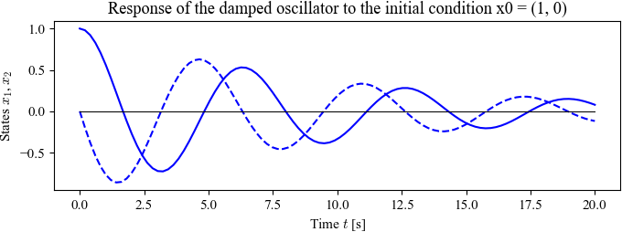
Figure 5.1: Response of a damped oscillator
Jump to navigation
Jump to search
| Chapter | Dynamic Behavior |
|---|---|
| Figure number | 5.1 |
| Figure title | Response of the damped oscillator to the initial condition x0 = (1, 0). |
| GitHub URL | https://github.com/murrayrm/fbs2e-python/blob/main/figure-5.1-damposc response.py |
| Requires | python-control |
Figure 5.1: Response of the damped oscillator to the initial condition x0 = (1, 0). The solution is unique for the given initial conditions and consists of an oscillatory solution for each state, with an exponentially decaying magnitude.
# damposc_response.py - dampled oscillator response
# RMM, 28 May 2023

import matplotlib.pyplot as plt
import numpy as np
import control as ct
import fbs                      # FBS plotting customizations

# Oscillator parameters
damposc_params = {'m': 1, 'b': 0.2, 'k': 1}

# System model (as ODE)
def damposc_update(t, x, u, params):
    m, b, k = params['m'], params['b'], params['k']
    return np.array([x[1], -k/m * x[0] - b/m * x[1]])
damposc = ct.NonlinearIOSystem(damposc_update, params=damposc_params)

# Simulate the response
tvec = np.linspace(0, 20, 100)
response = ct.input_output_response(damposc, tvec, 0, X0=[1, 0])

# Plot the states
fbs.figure('211')
plt.plot(response.time, response.states[0], 'b-')
plt.plot(response.time, response.states[1], 'b--')
plt.plot([response.time[0], response.time[-1]], [0, 0], 'k-', linewidth=0.75)
plt.xlabel('Time $t$ [s]')
plt.ylabel('States $x_1$, $x_2$')
plt.title(
    "Response of the damped oscillator to the initial condition x0 = (1, 0)")
fbs.savefig('figure-5.1-damposc_response-time.png')
