Cruise control
This page documents the cruise control system that is used as a running example throughout the text. A detailed description of the dynamics of this system are presented in Chapter 4 - Examples. This page contains a description of the system, including the models and commands used to generate some of the plots in the text.
Introduction
Cruise control is the term used to describe a control system that regulates the speed of an automobile. Cruise control was commercially introduced in 1958 as an option on the Chrysler Imperial. The basic operation of a cruise controller is to sense the speed of the vehicle, compare this speed to a desired reference, and then accelerate or decelerate the car as required. The figure to the right shows a block diagram of this feedback system.
A simple control algorithm for controlling the speed is to use a "proportional plus integral" feedback. In this algorithm, we choose the amount of gas flowing to the engine based on both the error between the current and desired speed, and the integral of that error.
The plot on the right shows the results of this feedback for a step change in the desired speed and a variety of different masses for the car (which might result from having a different number of passengers or towing a trailer). Notice that independent of the mass (which varies by a factor of 3), the steady state speed of the vehicle always approaches the desired speed and achieves that speed within approximately 5 seconds. Thus the performance of the system is robust with respect to this uncertainty.
Dynamic model
To develop a mathematical model we start with a force balance for the car body. Let <amsmath>v</amsmath> be the speed of the car, <amsmath>m</amsmath> the total mass (including passengers), <amsmath>F</amsmath> the force generated by the contact of the wheels with the road, and <amsmath>F_d</amsmath> the disturbance force due to gravity, friction and aerodynamic drag. The equation of motion of the car is simply
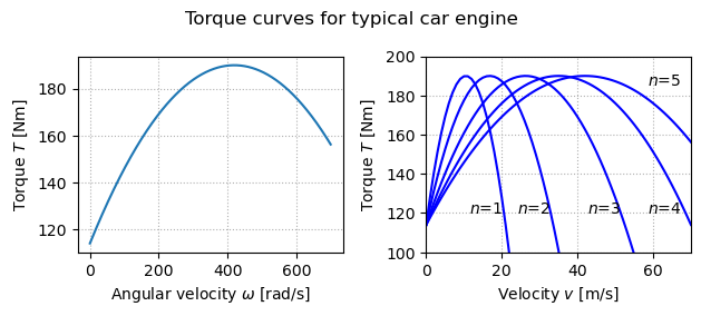
The force <amsmath>F</amsmath> is generated by the engine, whose torque is proportional to the rate of fuel injection, which is itself proportional to a control signal <amsmath>0 \leq u \leq 1</amsmath> that controls the throttle position. The torque also depends on engine speed <amsmath>\omega</amsmath>. A simple representation of the torque at full throttle is given by the torque curve
 T(\omega) = T_m \left(1 - \beta \biggl(\frac{\omega}{\omega_m} - 1\biggr)^2
 \right),
 \label{eq:cruise:torque}
</amsmath>where the maximum torque <amsmath>T_m</amsmath> is obtained at engine speed <amsmath>\omega_m</amsmath>. Typical parameters are <amsmath>T_m = 190</amsmath> Nm, <amsmath>\omega_m</amsmath> = 420 rad/s (about 4000 RPM) and <amsmath>\beta = 0.4</amsmath>.
Let <amsmath>n</amsmath> be the gear ratio and <amsmath>r</amsmath> the wheel radius. The engine speed is related to the velocity through the expression
\omega = \frac{n}{r} v =: \alpha_n v,
</amsmath>and the driving force can be written as
F = \frac{nu}{r} T(\omega) = \alpha_n u T(\alpha_n v).
</amsmath>Typical values of <amsmath>\alpha_n</amsmath> for gears 1 through 5 are <amsmath>\alpha_1 = 40</amsmath>, <amsmath>\alpha_2 = 25</amsmath>, <amsmath>\alpha_3 = 16</amsmath>, <amsmath>\alpha_4 = 12</amsmath> and <amsmath>\alpha_5 = 10</amsmath>. The inverse of <amsmath>\alpha_n</amsmath> has a physical interpretation as the effective wheel radius. The figure to the right shows the torque as a function of vehicle speed. The figure shows that the effect of the gear is to "flatten" the torque curve so that an almost full torque can be obtained almost over the whole speed range.
The disturbance force <amsmath>F_d</amsmath> has three major components: <amsmath>F_g</amsmath>, the forces due to gravity; <amsmath>F_r</amsmath>, the forces due to rolling friction; and <amsmath>F_a</amsmath>, the aerodynamic drag. Letting the slope of the road be <amsmath>\theta</amsmath>, gravity gives the force <amsmath>F_g = m g \sin\theta</amsmath>, where <amsmath>g = 9.8\, \text{m}/\text{s}^2</amsmath> is the gravitational constant. A simple model of rolling friction is
F_r = m g C_r\, \text{sgn}(v),
</amsmath>where <amsmath>C_r</amsmath> is the coefficient of rolling friction and sgn(<amsmath>v</amsmath>) is the sign of <amsmath>v</amsmath> or zero if <amsmath>v = 0</amsmath>. A typical value for the coefficient of rolling friction is <amsmath>C_r = 0.01</amsmath>. Finally, the aerodynamic drag is proportional to the square of the speed:
F_a = \frac{1}{2} \rho C_d A v^2,
</amsmath>where <amsmath>\rho</amsmath> is the density of air, <amsmath>C_d</amsmath> is the shape-dependent aerodynamic drag coefficient and <amsmath>A</amsmath> is the frontal area of the car. Typical parameters are <amsmath>\rho = </amsmath> 1.3 k/m<amsmath>{}^3</amsmath>, <amsmath>C_d = 0.32</amsmath> and <amsmath>A =</amsmath> 2.4 m<amsmath>{}^2</amsmath>.
SIMULINK model
The file Template:Matlabfile contains a nonlinear model of a cruise controller for a car, depicted below.
The model contains all of the dynamics described in Section 3.1.
MATLAB model
An alternative model for the system is a MATLAB model suitable for use with the 'ode45' function. The file Template:Matlabfile contains a nonlinear model of the car dynamics consistent with the description given in Section 3.1.
MATLAB files
A number of MATLAB files are available that correspond to examples in the printed text. This section contains links to the various files that are available. Note that you will also need some of the MATLAB tools.
Standalone versions of the model:
- Template:Am08 matlab - SIMULINK model for cruise controller in Section 3.1
- Template:Am08 matlab - MATLAB function to compute the acceleration given the vehicle state, inputs and parameters
Linearized models (all files required):
- Template:Am08 matlab - Parameters for car model
- Template:Am08 matlab - Defines default operating condition
- Template:Am08 matlab - Linearized model of the car dynamics
- Template:Am08 matlab - Parameters for PI controller (including anti-windup)
- Template:Am08 matlab - Closed loop dynamics for linear and nonlinear models (including anti-windup)
Controller designs (require linearized models):
- Template:Am08 matlab - Basic proportional plus integral controller (Example 5.1)
- Template:Am08 matlab - State feedback controller, with integral action (Example 6.10)
- Template:Am08 matlab - PI controller with antiwindup compensation (Example 10.5)
Exercises
The following exercises make use of the cruise control model described here:
Further Reading
- How Stuff Works: cruise control
- Wikipedia: cruise control

