Difference between revisions of "Figure 5.7: Phase portrait and time domain simulation for a system with a single stable equilibrium point"
Jump to navigation
Jump to search
| Line 9: | Line 9: | ||
|- | |- | ||
| rowspan=3 | [[Image:figure-5.7-stable_eqpt-pp.png]] | | rowspan=3 | [[Image:figure-5.7-stable_eqpt-pp.png]] | ||
| − | | <math> \dot x_1 &= x_2 \\ \dot x_2 &= -x_1 </math> | + | | <math> \begin{aligned} \dot x_1 &= x_2 \\ \dot x_2 &= -x_1 \end{aligned} </math> |
|- | |- | ||
| rowspan=2 | [[Image:figure-5.7-stable_eqpt-time.png]] | | rowspan=2 | [[Image:figure-5.7-stable_eqpt-time.png]] | ||
Revision as of 05:37, 7 April 2024
| Chapter | Dynamic Behavior |
|---|---|
| Figure number | 5.7 |
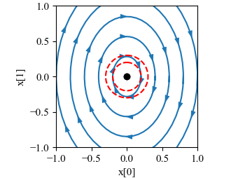
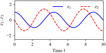
| Figure title | 5.7: Phase portrait and time domain simulation for a system with a single stable equilibrium point |
| GitHub URL | https://github.com/murrayrm/fbs2e-python/blob/main/figure-5.7-stable-eqpt.py |
| Requires | python-control |

|
|

|
Figure 5.7: Phase portrait and time domain simulation for a system with a single stable equilibrium point. The equilibrium point $x_\text{e}$ at the origin is stable since all trajectories that start near $x_\text{e}$ stay near $x_\text{e}$.
