Difference between revisions of "Figure 5.3: Phase portraits"
Jump to navigation
Jump to search
m |
|||
| Line 30: | Line 30: | ||
damposc = ct.nlsys(damposc_update, states=2, params=damposc_params) | damposc = ct.nlsys(damposc_update, states=2, params=damposc_params) | ||
| − | # Set the | + | # Set the limits for the plot |
limits = [-1, 1, -1, 1] | limits = [-1, 1, -1, 1] | ||
Latest revision as of 01:09, 7 April 2024
| Chapter | Dynamic Behavior |
|---|---|
| Figure number | 5.3 |
| Figure title | Phase portraits |
| GitHub URL | https://github.com/murrayrm/fbs2e-python/blob/main/figure-5.3-phase portraits.py |
| Requires | python-control |
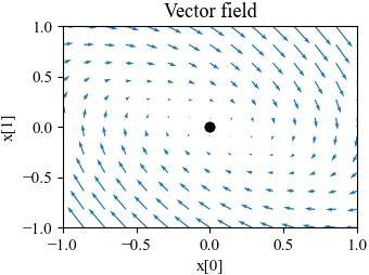
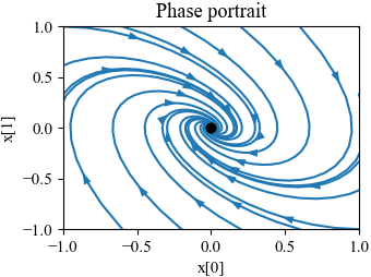
Figure 5.3: Phase portraits. (a) This plot shows the vector field for a planar dynamical system. Each arrow shows the velocity at that point in the state space. (b) This plot includes the solutions (sometimes called streamlines) from different initial conditions, with the vector field superimposed.
# phase_portraits.py - phase portrait examples
# RMM, 6 Apr 2024

import matplotlib.pyplot as plt
import numpy as np
import control as ct
import control.phaseplot as pp
import fbs                      # FBS plotting customizations

# Oscillator parameters
damposc_params = {'m': 1, 'b': 1, 'k': 1}

# System model (as ODE)
def damposc_update(t, x, u, params):
    m, b, k = params['m'], params['b'], params['k']
    return np.array([x[1], -k/m * x[0] - b/m * x[1]])
damposc = ct.nlsys(damposc_update, states=2, params=damposc_params)

# Set the limits for the plot
limits = [-1, 1, -1, 1]

# Vector field
fbs.figure('mlh')
ct.phase_plane_plot(
    damposc, limits, plot_streamlines=False,
    plot_vectorfield=True, gridspec=[15, 12])
plt.suptitle(""); plt.title("Vector field")
fbs.savefig('figure-5.3-phase_portraits-vf.png')

# Streamlines
fbs.figure('mlh')
ct.phase_plane_plot(damposc, limits, 8)
plt.suptitle(""); plt.title("Phase portrait")
fbs.savefig('figure-5.3-phase_portraits-sl.png')

