Difference between revisions of "Cruise control"
| Line 53: | Line 53: | ||
{{Code block|Package initialization}} | {{Code block|Package initialization}} | ||
{{Code start}} | {{Code start}} | ||
| − | + | import numpy as np | |
| − | + | import matplotlib.pyplot as plt | |
| − | + | from math import pi | |
| − | + | import control as ct | |
{{Code end}} | {{Code end}} | ||
{{Code block|Vehicle model}} | {{Code block|Vehicle model}} | ||
{{Code start}} | {{Code start}} | ||
| − | + | def vehicle_update(t, x, u, params={}): | |
| − | + | """Vehicle dynamics for cruise control system. | |
| − | + | ||
| − | + | Parameters | |
| − | + | ---------- | |
| − | + | x : array | |
| − | + | System state: car velocity in m/s | |
| − | + | u : array | |
| − | + | System input: [throttle, gear, road_slope], where throttle is | |
| − | + | a float between 0 and 1, gear is an integer between 1 and 5, | |
| − | + | and road_slope is in rad. | |
| − | + | ||
| − | + | Returns | |
| − | + | ------- | |
| − | + | float | |
| − | + | Vehicle acceleration | |
| − | + | """ | |
| − | + | ||
| − | + | from math import copysign, sin | |
| − | + | sign = lambda x: copysign(1, x) # define the sign() function | |
| − | + | ||
| − | + | # Set up the system parameters | |
| − | + | m = params.get('m', 1600.) # vehicle mass, kg | |
| − | + | g = params.get('g', 9.8) # gravitational constant, m/s^2 | |
| − | + | Cr = params.get('Cr', 0.01) # coefficient of rolling friction | |
| − | + | Cd = params.get('Cd', 0.32) # drag coefficient | |
| − | + | rho = params.get('rho', 1.3) # density of air, kg/m^3 | |
| − | + | A = params.get('A', 2.4) # car area, m^2 | |
| − | + | alpha = params.get( | |
| − | + | 'alpha', [40, 25, 16, 12, 10]) # gear ratio / wheel radius | |
| − | + | ||
| − | + | # Define variables for vehicle state and inputs | |
| − | + | v = x[0] # vehicle velocity | |
| − | + | throttle = np.clip(u[0], 0, 1) # vehicle throttle | |
| − | + | gear = u[1] # vehicle gear | |
| − | + | theta = u[2] # road slope | |
| − | + | ||
| − | + | # Force generated by the engine | |
| − | + | omega = alpha[int(gear)-1] * v # engine angular speed | |
| − | + | F = alpha[int(gear)-1] * motor_torque(omega, params) * throttle | |
| − | + | ||
| − | + | # Disturbance forces | |
| − | + | # | |
| − | + | # The disturbance force Fd has three major components: Fg, the forces due | |
| − | + | # to gravity; Fr, the forces due to rolling friction; and Fa, the | |
| − | + | # aerodynamic drag. | |
| − | + | ||
| − | + | # Letting the slope of the road be \theta (theta), gravity gives the | |
| − | + | # force Fg = m g sin \theta. | |
| − | + | Fg = m * g * sin(theta) | |
| − | + | ||
| − | + | # A simple model of rolling friction is Fr = m g Cr sgn(v), where Cr is | |
| − | + | # the coefficient of rolling friction and sgn(v) is the sign of v (±1) or | |
| − | + | # zero if v = 0. | |
| − | + | Fr = m * g * Cr * sign(v) | |
| − | + | ||
| − | + | # The aerodynamic drag is proportional to the square of the speed: Fa = | |
| − | + | # 1/2 \rho Cd A |v| v, where \rho is the density of air, Cd is the | |
| − | + | # shape-dependent aerodynamic drag coefficient, and A is the frontal area | |
| − | + | # of the car. | |
| − | + | Fa = 1/2 * rho * Cd * A * abs(v) * v | |
| − | + | ||
| − | + | # Final acceleration on the car | |
| − | + | Fd = Fg + Fr + Fa | |
| − | + | dv = (F - Fd) / m | |
| − | + | ||
| − | + | return dv | |
{{Code end}} | {{Code end}} | ||
{{Code block|Engine model}} | {{Code block|Engine model}} | ||
{{Code start}} | {{Code start}} | ||
| − | + | def motor_torque(omega, params={}): | |
| − | + | # Set up the system parameters | |
| − | + | Tm = params.get('Tm', 190.) # engine torque constant | |
| − | + | omega_m = params.get('omega_m', 420.) # peak engine angular speed | |
| − | + | beta = params.get('beta', 0.4) # peak engine rolloff | |
| − | + | ||
| − | + | return np.clip(Tm * (1 - beta * (omega/omega_m - 1)**2), 0, None) | |
{{Code end}} | {{Code end}} | ||
{{Code block|Input/output model for the vehicle system}} | {{Code block|Input/output model for the vehicle system}} | ||
{{Code start}} | {{Code start}} | ||
| − | + | vehicle = ct.NonlinearIOSystem( | |
| − | + | vehicle_update, None, name='vehicle', | |
| − | + | inputs = ('u', 'gear', 'theta'), outputs = ('v'), states=('v')) | |
| − | + | {Code end}} | |
{{Code block|Input/output torque curves (plot)}} | {{Code block|Input/output torque curves (plot)}} | ||
{{Code start}} | {{Code start}} | ||
| − | + | # Figure 4.2a - single torque curve as function of omega | |
| − | + | omega_range = np.linspace(0, 700, 701) | |
| − | + | plt.subplot(2, 2, 1) | |
| − | + | plt.plot(omega_range, [motor_torque(w) for w in omega_range]) | |
| − | + | plt.xlabel('Angular velocity $\omega$ [rad/s]') | |
| − | + | plt.ylabel('Torque $T$ [Nm]') | |
| − | + | plt.grid(True, linestyle='dotted') | |
| − | + | ||
| − | + | # Figure 4.2b - torque curves in different gears, as function of velocity | |
| − | + | plt.subplot(2, 2, 2) | |
| − | + | v_range = np.linspace(0, 70, 71) | |
| − | + | alpha = [40, 25, 16, 12, 10] | |
| − | + | for gear in range(5): | |
| − | + | omega_range = alpha[gear] * v_range | |
| − | + | plt.plot(v_range, [motor_torque(w) for w in omega_range], | |
| − | + | color='blue', linestyle='solid') | |
| − | + | ||
| − | + | # Set up the axes and style | |
| − | + | plt.axis([0, 70, 100, 200]) | |
| − | + | plt.grid(True, linestyle='dotted') | |
| − | + | ||
| − | + | # Add labels | |
| − | + | plt.text(11.5, 120, '$n$=1') | |
| − | + | plt.text(24, 120, '$n$=2') | |
| − | + | plt.text(42.5, 120, '$n$=3') | |
| − | + | plt.text(58.5, 120, '$n$=4') | |
| − | + | plt.text(58.5, 185, '$n$=5') | |
| − | + | plt.xlabel('Velocity $v$ [m/s]') | |
| − | + | plt.ylabel('Torque $T$ [Nm]') | |
| − | + | ||
| − | + | plt.suptitle('Torque curves for typical car engine'); | |
| − | + | plt.tight_layout() | |
{{Code end}} | {{Code end}} | ||
{{Code block|PI controller}} | {{Code block|PI controller}} | ||
{{Code start}} | {{Code start}} | ||
| − | + | # Construct a PI controller with rolloff, as a transfer function | |
| − | + | Kp = 0.5 # proportional gain | |
| − | + | Ki = 0.1 # integral gain | |
| − | + | control_pi = ct.tf2io( | |
| − | + | ct.TransferFunction([Kp, Ki], [1, 0.01*Ki/Kp]), | |
| − | + | name='control', inputs='u', outputs='y') | |
| − | + | ||
| − | + | cruise_pi = ct.InterconnectedSystem( | |
| − | + | (vehicle, control_pi), name='cruise', | |
| − | + | connections = [('control.u', '-vehicle.v'), ('vehicle.u', 'control.y')], | |
| − | + | inplist = ('control.u', 'vehicle.gear', 'vehicle.theta'), inputs = ('vref', 'gear', 'theta'), | |
| − | + | outlist = ('vehicle.v', 'vehicle.u'), outputs = ('v', 'u')) | |
{{Code end}} | {{Code end}} | ||
{{Code block|Plotting function}} | {{Code block|Plotting function}} | ||
{{Code start}} | {{Code start}} | ||
| − | + | # Define a generator for creating a "standard" cruise control plot | |
| − | + | def cruise_plot(sys, t, y, t_hill=5, vref=20, antiwindup=False, linetype='b-', | |
| − | + | subplots=[None, None]): | |
| − | + | # Figure out the plot bounds and indices | |
| − | + | v_min = vref-1.2; v_max = vref+0.5; v_ind = sys.find_output('v') | |
| − | + | u_min = 0; u_max = 2 if antiwindup else 1; u_ind = sys.find_output('u') | |
| − | + | ||
| − | + | # Make sure the upper and lower bounds on v are OK | |
| − | + | while max(y[v_ind]) > v_max: v_max += 1 | |
| − | + | while min(y[v_ind]) < v_min: v_min -= 1 | |
| − | + | ||
| − | + | # Create arrays for return values | |
| − | + | subplot_axes = subplots.copy() | |
| − | + | ||
| − | + | # Velocity profile | |
| − | + | if subplot_axes[0] is None: | |
| − | + | subplot_axes[0] = plt.subplot(2, 1, 1) | |
| − | + | else: | |
| − | + | plt.sca(subplots[0]) | |
| − | + | plt.plot(t, y[v_ind], linetype) | |
| − | + | plt.plot(t, vref*np.ones(t.shape), 'k-') | |
| − | + | plt.plot([t_hill, t_hill], [v_min, v_max], 'k--') | |
| − | + | plt.axis([0, t[-1], v_min, v_max]) | |
| − | + | plt.xlabel('Time $t$ [s]') | |
| − | + | plt.ylabel('Velocity $v$ [m/s]') | |
| − | + | ||
| − | + | # Commanded input profile | |
| − | + | if subplot_axes[1] is None: | |
| − | + | subplot_axes[1] = plt.subplot(2, 1, 2) | |
| − | + | else: | |
| − | + | plt.sca(subplots[1]) | |
| − | + | plt.plot(t, y[u_ind], 'r--' if antiwindup else linetype) | |
| − | + | plt.plot([t_hill, t_hill], [u_min, u_max], 'k--') | |
| − | + | plt.axis([0, t[-1], u_min, u_max]) | |
| − | + | plt.xlabel('Time $t$ [s]') | |
| − | + | plt.ylabel('Throttle $u$') | |
| − | + | ||
| − | + | # Applied input profile | |
| − | + | if antiwindup: | |
| − | + | plt.plot(t, np.clip(y[u_ind], 0, 1), linetype) | |
| − | + | plt.legend(['Commanded', 'Applied'], frameon=False) | |
| − | + | ||
| − | + | return subplot_axes | |
{{Code end}} | {{Code end}} | ||
{{Code block|Simulated responses}} | {{Code block|Simulated responses}} | ||
{{Code start}} | {{Code start}} | ||
| − | + | # Define the time and input vectors | |
| − | + | T = np.linspace(0, 25, 101) | |
| − | + | vref = 20 * np.ones(T.shape) | |
| − | + | gear = 4 * np.ones(T.shape) | |
| − | + | theta0 = np.zeros(T.shape) | |
| − | + | ||
| − | + | # Now simulate the effect of a hill at t = 5 seconds | |
| − | + | plt.figure() | |
| − | + | plt.suptitle('Response to change in road slope') | |
| − | + | theta_hill = np.array([ | |
| − | + | 0 if t <= 5 else | |
| − | + | 4./180. * pi * (t-5) if t <= 6 else | |
| − | + | 4./180. * pi for t in T]) | |
| − | + | ||
| − | + | subplots = [None, None] | |
| − | + | linecolor = ['red', 'blue', 'green'] | |
| − | + | handles = [] | |
| − | + | for i, m in enumerate([1200, 1600, 2000]): | |
| − | + | # Compute the equilibrium state for the system | |
| − | + | X0, U0 = ct.find_eqpt( | |
| − | + | cruise_tf, [vref[0], 0], [vref[0], gear[0], theta0[0]], | |
| − | + | iu=[1, 2], y0=[vref[0], 0], iy=[0], params={'m':m}) | |
| − | + | ||
| − | + | t, y = ct.input_output_response( | |
| − | + | cruise_tf, T, [vref, gear, theta_hill], X0, params={'m':m}) | |
| − | + | ||
| − | + | subplots = cruise_plot(cruise_tf, t, y, t_hill=5, subplots=subplots, | |
| − | + | linetype=linecolor[i][0] + '-') | |
| − | + | handles.append(mlines.Line2D([], [], color=linecolor[i], linestyle='-', | |
| − | + | label="m = %d" % m)) | |
| − | + | ||
| − | + | # Add labels to the plots | |
| − | + | plt.sca(subplots[0]) | |
| − | + | plt.ylabel('Speed [m/s]') | |
| − | + | plt.legend(handles=handles, frameon=False, loc='lower right'); | |
| − | + | ||
| − | + | plt.sca(subplots[1]) | |
| − | + | plt.ylabel('Throttle') | |
| − | + | plt.xlabel('Time [s]'); | |
{{Code end}} | {{Code end}} | ||
Revision as of 17:50, 29 December 2020
This page documents the cruise control system that is used as a running example throughout the text. A detailed description of the dynamics of this system are presented in Chapter 4 - Examples. This page contains a description of the system, including the models and commands used to generate some of the plots in the text.
Introduction

Cruise control is the term used to describe a control system that regulates the speed of an automobile. Cruise control was commercially introduced in 1958 as an option on the Chrysler Imperial. The basic operation of a cruise controller is to sense the speed of the vehicle, compare this speed to a desired reference, and then accelerate or decelerate the car as required. The figure to the right shows a block diagram of this feedback system.
A simple control algorithm for controlling the speed is to use a "proportional plus integral" feedback. In this algorithm, we choose the amount of gas flowing to the engine based on both the error between the current and desired speed, and the integral of that error. The plot on the right shows the results of this feedback for a step change in the desired speed and a variety of different masses for the car (which might result from having a different number of passengers or towing a trailer). Notice that independent of the mass (which varies by 25% of the total weight of the car), the steady state speed of the vehicle always approaches the desired speed and achieves that speed within approximately 10-15 seconds. Thus the performance of the system is robust with respect to this uncertainty.
Dynamic model
To develop a mathematical model we start with a force balance for the car body. Let Failed to parse (MathML with SVG or PNG fallback (recommended for modern browsers and accessibility tools): Invalid response ("Math extension cannot connect to Restbase.") from server "https://en.wikipedia.org/api/rest_v1/":): {\displaystyle v} be the speed of the car, Failed to parse (MathML with SVG or PNG fallback (recommended for modern browsers and accessibility tools): Invalid response ("Math extension cannot connect to Restbase.") from server "https://en.wikipedia.org/api/rest_v1/":): {\displaystyle m} the total mass (including passengers), the force generated by the contact of the wheels with the road, and the disturbance force due to gravity, friction and aerodynamic drag. The equation of motion of the car is simply


The force Failed to parse (MathML with SVG or PNG fallback (recommended for modern browsers and accessibility tools): Invalid response ("Math extension cannot connect to Restbase.") from server "https://en.wikipedia.org/api/rest_v1/":): {\displaystyle F} is generated by the engine, whose torque is proportional to the rate of fuel injection, which is itself proportional to a control signal Failed to parse (MathML with SVG or PNG fallback (recommended for modern browsers and accessibility tools): Invalid response ("Math extension cannot connect to Restbase.") from server "https://en.wikipedia.org/api/rest_v1/":): {\displaystyle 0 \leq u \leq 1} that controls the throttle position. The torque also depends on engine speed Failed to parse (MathML with SVG or PNG fallback (recommended for modern browsers and accessibility tools): Invalid response ("Math extension cannot connect to Restbase.") from server "https://en.wikipedia.org/api/rest_v1/":): {\displaystyle \omega} . A simple representation of the torque at full throttle is given by the torque curve
where the maximum torque Failed to parse (MathML with SVG or PNG fallback (recommended for modern browsers and accessibility tools): Invalid response ("Math extension cannot connect to Restbase.") from server "https://en.wikipedia.org/api/rest_v1/":): {\displaystyle T_\text{m}} is obtained at engine speed Failed to parse (MathML with SVG or PNG fallback (recommended for modern browsers and accessibility tools): Invalid response ("Math extension cannot connect to Restbase.") from server "https://en.wikipedia.org/api/rest_v1/":): {\displaystyle \omega_\text{m}} . Typical parameters are Failed to parse (MathML with SVG or PNG fallback (recommended for modern browsers and accessibility tools): Invalid response ("Math extension cannot connect to Restbase.") from server "https://en.wikipedia.org/api/rest_v1/":): {\displaystyle T_m = 190} Nm, Failed to parse (MathML with SVG or PNG fallback (recommended for modern browsers and accessibility tools): Invalid response ("Math extension cannot connect to Restbase.") from server "https://en.wikipedia.org/api/rest_v1/":): {\displaystyle \omega_m} = 420 rad/s (about 4000 RPM) and Failed to parse (MathML with SVG or PNG fallback (recommended for modern browsers and accessibility tools): Invalid response ("Math extension cannot connect to Restbase.") from server "https://en.wikipedia.org/api/rest_v1/":): {\displaystyle \beta = 0.4} .
Let Failed to parse (MathML with SVG or PNG fallback (recommended for modern browsers and accessibility tools): Invalid response ("Math extension cannot connect to Restbase.") from server "https://en.wikipedia.org/api/rest_v1/":): {\displaystyle n} be the gear ratio and Failed to parse (MathML with SVG or PNG fallback (recommended for modern browsers and accessibility tools): Invalid response ("Math extension cannot connect to Restbase.") from server "https://en.wikipedia.org/api/rest_v1/":): {\displaystyle r} the wheel radius. The engine speed is related to the velocity through the expression
and the driving force can be written as

Typical values of Failed to parse (MathML with SVG or PNG fallback (recommended for modern browsers and accessibility tools): Invalid response ("Math extension cannot connect to Restbase.") from server "https://en.wikipedia.org/api/rest_v1/":): {\displaystyle \alpha_n} for gears 1 through 5 are Failed to parse (MathML with SVG or PNG fallback (recommended for modern browsers and accessibility tools): Invalid response ("Math extension cannot connect to Restbase.") from server "https://en.wikipedia.org/api/rest_v1/":): {\displaystyle \alpha_1 = 40} , Failed to parse (MathML with SVG or PNG fallback (recommended for modern browsers and accessibility tools): Invalid response ("Math extension cannot connect to Restbase.") from server "https://en.wikipedia.org/api/rest_v1/":): {\displaystyle \alpha_2 = 25} , Failed to parse (MathML with SVG or PNG fallback (recommended for modern browsers and accessibility tools): Invalid response ("Math extension cannot connect to Restbase.") from server "https://en.wikipedia.org/api/rest_v1/":): {\displaystyle \alpha_3 = 16} , and Failed to parse (MathML with SVG or PNG fallback (recommended for modern browsers and accessibility tools): Invalid response ("Math extension cannot connect to Restbase.") from server "https://en.wikipedia.org/api/rest_v1/":): {\displaystyle \alpha_5 = 10} . The inverse of Failed to parse (MathML with SVG or PNG fallback (recommended for modern browsers and accessibility tools): Invalid response ("Math extension cannot connect to Restbase.") from server "https://en.wikipedia.org/api/rest_v1/":): {\displaystyle \alpha_n} has a physical interpretation as the effective wheel radius. The figure to the right shows the torque as a function of vehicle speed. The figure shows that the effect of the gear is to "flatten" the torque curve so that an almost full torque can be obtained almost over the whole speed range.

The disturbance force Failed to parse (MathML with SVG or PNG fallback (recommended for modern browsers and accessibility tools): Invalid response ("Math extension cannot connect to Restbase.") from server "https://en.wikipedia.org/api/rest_v1/":): {\displaystyle F_\text{d}} has three major components: Failed to parse (MathML with SVG or PNG fallback (recommended for modern browsers and accessibility tools): Invalid response ("Math extension cannot connect to Restbase.") from server "https://en.wikipedia.org/api/rest_v1/":): {\displaystyle F_\text{g}} , the forces due to gravity; Failed to parse (MathML with SVG or PNG fallback (recommended for modern browsers and accessibility tools): Invalid response ("Math extension cannot connect to Restbase.") from server "https://en.wikipedia.org/api/rest_v1/":): {\displaystyle F_\text{r}} , the forces due to rolling friction; and Failed to parse (MathML with SVG or PNG fallback (recommended for modern browsers and accessibility tools): Invalid response ("Math extension cannot connect to Restbase.") from server "https://en.wikipedia.org/api/rest_v1/":): {\displaystyle F_\text{a}} , the aerodynamic drag. Letting the slope of the road be Failed to parse (MathML with SVG or PNG fallback (recommended for modern browsers and accessibility tools): Invalid response ("Math extension cannot connect to Restbase.") from server "https://en.wikipedia.org/api/rest_v1/":): {\displaystyle \theta} , gravity gives the force Failed to parse (MathML with SVG or PNG fallback (recommended for modern browsers and accessibility tools): Invalid response ("Math extension cannot connect to Restbase.") from server "https://en.wikipedia.org/api/rest_v1/":): {\displaystyle F_\text{g} = m g \sin\theta} , where Failed to parse (MathML with SVG or PNG fallback (recommended for modern browsers and accessibility tools): Invalid response ("Math extension cannot connect to Restbase.") from server "https://en.wikipedia.org/api/rest_v1/":): {\displaystyle g = 9.8\, \text{m}/\text{s}^2} is the gravitational constant. A simple model of rolling friction is
where Failed to parse (MathML with SVG or PNG fallback (recommended for modern browsers and accessibility tools): Invalid response ("Math extension cannot connect to Restbase.") from server "https://en.wikipedia.org/api/rest_v1/":): {\displaystyle C_\text{r}} is the coefficient of rolling friction and sgn(Failed to parse (MathML with SVG or PNG fallback (recommended for modern browsers and accessibility tools): Invalid response ("Math extension cannot connect to Restbase.") from server "https://en.wikipedia.org/api/rest_v1/":): {\displaystyle v} ) is the sign of Failed to parse (MathML with SVG or PNG fallback (recommended for modern browsers and accessibility tools): Invalid response ("Math extension cannot connect to Restbase.") from server "https://en.wikipedia.org/api/rest_v1/":): {\displaystyle v} or zero if Failed to parse (MathML with SVG or PNG fallback (recommended for modern browsers and accessibility tools): Invalid response ("Math extension cannot connect to Restbase.") from server "https://en.wikipedia.org/api/rest_v1/":): {\displaystyle v = 0} . A typical value for the coefficient of rolling friction is Failed to parse (MathML with SVG or PNG fallback (recommended for modern browsers and accessibility tools): Invalid response ("Math extension cannot connect to Restbase.") from server "https://en.wikipedia.org/api/rest_v1/":): {\displaystyle C_\text{r} = 0.01} . Finally, the aerodynamic drag is proportional to the square of the speed:
where Failed to parse (MathML with SVG or PNG fallback (recommended for modern browsers and accessibility tools): Invalid response ("Math extension cannot connect to Restbase.") from server "https://en.wikipedia.org/api/rest_v1/":): {\displaystyle \rho} is the density of air, Failed to parse (MathML with SVG or PNG fallback (recommended for modern browsers and accessibility tools): Invalid response ("Math extension cannot connect to Restbase.") from server "https://en.wikipedia.org/api/rest_v1/":): {\displaystyle C_d} is the shape-dependent aerodynamic drag coefficient and Failed to parse (MathML with SVG or PNG fallback (recommended for modern browsers and accessibility tools): Invalid response ("Math extension cannot connect to Restbase.") from server "https://en.wikipedia.org/api/rest_v1/":): {\displaystyle A} is the frontal area of the car. Typical parameters are Failed to parse (MathML with SVG or PNG fallback (recommended for modern browsers and accessibility tools): Invalid response ("Math extension cannot connect to Restbase.") from server "https://en.wikipedia.org/api/rest_v1/":): {\displaystyle \rho = } 1.3 k/mFailed to parse (MathML with SVG or PNG fallback (recommended for modern browsers and accessibility tools): Invalid response ("Math extension cannot connect to Restbase.") from server "https://en.wikipedia.org/api/rest_v1/":): {\displaystyle {}^3} , Failed to parse (MathML with SVG or PNG fallback (recommended for modern browsers and accessibility tools): Invalid response ("Math extension cannot connect to Restbase.") from server "https://en.wikipedia.org/api/rest_v1/":): {\displaystyle C_\text{d} = 0.32} and 2.4 mFailed to parse (MathML with SVG or PNG fallback (recommended for modern browsers and accessibility tools): Invalid response ("Math extension cannot connect to Restbase.") from server "https://en.wikipedia.org/api/rest_v1/":): {\displaystyle {}^2} .

Python code
The model for the system above can be built using the Python Control Toolbox. The code blocks in this section can be used to generate the plots above.
import numpy as np
import matplotlib.pyplot as plt
from math import pi
import control as ct
def vehicle_update(t, x, u, params={}):
    """Vehicle dynamics for cruise control system.

    Parameters
    ----------
    x : array
         System state: car velocity in m/s
    u : array
         System input: [throttle, gear, road_slope], where throttle is
         a float between 0 and 1, gear is an integer between 1 and 5,
         and road_slope is in rad.

    Returns
    -------
    float
        Vehicle acceleration
    """

    from math import copysign, sin
    sign = lambda x: copysign(1, x)         # define the sign() function

    # Set up the system parameters
    m = params.get('m', 1600.)              # vehicle mass, kg
    g = params.get('g', 9.8)                # gravitational constant, m/s^2
    Cr = params.get('Cr', 0.01)             # coefficient of rolling friction
    Cd = params.get('Cd', 0.32)             # drag coefficient
    rho = params.get('rho', 1.3)            # density of air, kg/m^3
    A = params.get('A', 2.4)                # car area, m^2
    alpha = params.get(
        'alpha', [40, 25, 16, 12, 10])      # gear ratio / wheel radius

    # Define variables for vehicle state and inputs
    v = x[0]                           # vehicle velocity
    throttle = np.clip(u[0], 0, 1)     # vehicle throttle
    gear = u[1]                        # vehicle gear
    theta = u[2]                       # road slope

    # Force generated by the engine
    omega = alpha[int(gear)-1] * v      # engine angular speed
    F = alpha[int(gear)-1] * motor_torque(omega, params) * throttle

    # Disturbance forces
    #
    # The disturbance force Fd has three major components: Fg, the forces due
    # to gravity; Fr, the forces due to rolling friction; and Fa, the
    # aerodynamic drag.

    # Letting the slope of the road be \theta (theta), gravity gives the
    # force Fg = m g sin \theta.
    Fg = m * g * sin(theta)

    # A simple model of rolling friction is Fr = m g Cr sgn(v), where Cr is
    # the coefficient of rolling friction and sgn(v) is the sign of v (±1) or
    # zero if v = 0.
    Fr  = m * g * Cr * sign(v)

    # The aerodynamic drag is proportional to the square of the speed: Fa =
    # 1/2 \rho Cd A |v| v, where \rho is the density of air, Cd is the
    # shape-dependent aerodynamic drag coefficient, and A is the frontal area
    # of the car.
    Fa = 1/2 * rho * Cd * A * abs(v) * v

    # Final acceleration on the car
    Fd = Fg + Fr + Fa
    dv = (F - Fd) / m

    return dv
def motor_torque(omega, params={}):
    # Set up the system parameters
    Tm = params.get('Tm', 190.)             # engine torque constant
    omega_m = params.get('omega_m', 420.)   # peak engine angular speed
    beta = params.get('beta', 0.4)          # peak engine rolloff

    return np.clip(Tm * (1 - beta * (omega/omega_m - 1)**2), 0, None)
vehicle = ct.NonlinearIOSystem(
vehicle_update, None, name='vehicle',
inputs = ('u', 'gear', 'theta'), outputs = ('v'), states=('v'))
{Code end}}
Input/output torque curves (plot)
# Figure 4.2a - single torque curve as function of omega
omega_range = np.linspace(0, 700, 701)
plt.subplot(2, 2, 1)
plt.plot(omega_range, [motor_torque(w) for w in omega_range])
plt.xlabel('Angular velocity $\omega$ [rad/s]')
plt.ylabel('Torque $T$ [Nm]')
plt.grid(True, linestyle='dotted')
# Figure 4.2b - torque curves in different gears, as function of velocity
plt.subplot(2, 2, 2)
v_range = np.linspace(0, 70, 71)
alpha = [40, 25, 16, 12, 10]
for gear in range(5):
omega_range = alpha[gear] * v_range
plt.plot(v_range, [motor_torque(w) for w in omega_range],
color='blue', linestyle='solid')
# Set up the axes and style
plt.axis([0, 70, 100, 200])
plt.grid(True, linestyle='dotted')
# Add labels
plt.text(11.5, 120, '$n$=1')
plt.text(24, 120, '$n$=2')
plt.text(42.5, 120, '$n$=3')
plt.text(58.5, 120, '$n$=4')
plt.text(58.5, 185, '$n$=5')
plt.xlabel('Velocity $v$ [m/s]')
plt.ylabel('Torque $T$ [Nm]')
plt.suptitle('Torque curves for typical car engine');
plt.tight_layout()
PI controller
# Construct a PI controller with rolloff, as a transfer function
Kp = 0.5 # proportional gain
Ki = 0.1 # integral gain
control_pi = ct.tf2io(
ct.TransferFunction([Kp, Ki], [1, 0.01*Ki/Kp]),
name='control', inputs='u', outputs='y')
cruise_pi = ct.InterconnectedSystem(
(vehicle, control_pi), name='cruise',
connections = [('control.u', '-vehicle.v'), ('vehicle.u', 'control.y')],
inplist = ('control.u', 'vehicle.gear', 'vehicle.theta'), inputs = ('vref', 'gear', 'theta'),
outlist = ('vehicle.v', 'vehicle.u'), outputs = ('v', 'u'))
Plotting function
# Define a generator for creating a "standard" cruise control plot
def cruise_plot(sys, t, y, t_hill=5, vref=20, antiwindup=False, linetype='b-',
subplots=[None, None]):
# Figure out the plot bounds and indices
v_min = vref-1.2; v_max = vref+0.5; v_ind = sys.find_output('v')
u_min = 0; u_max = 2 if antiwindup else 1; u_ind = sys.find_output('u')
# Make sure the upper and lower bounds on v are OK
while max(y[v_ind]) > v_max: v_max += 1
while min(y[v_ind]) < v_min: v_min -= 1
# Create arrays for return values
subplot_axes = subplots.copy()
# Velocity profile
if subplot_axes[0] is None:
subplot_axes[0] = plt.subplot(2, 1, 1)
else:
plt.sca(subplots[0])
plt.plot(t, y[v_ind], linetype)
plt.plot(t, vref*np.ones(t.shape), 'k-')
plt.plot([t_hill, t_hill], [v_min, v_max], 'k--')
plt.axis([0, t[-1], v_min, v_max])
plt.xlabel('Time $t$ [s]')
plt.ylabel('Velocity $v$ [m/s]')
# Commanded input profile
if subplot_axes[1] is None:
subplot_axes[1] = plt.subplot(2, 1, 2)
else:
plt.sca(subplots[1])
plt.plot(t, y[u_ind], 'r--' if antiwindup else linetype)
plt.plot([t_hill, t_hill], [u_min, u_max], 'k--')
plt.axis([0, t[-1], u_min, u_max])
plt.xlabel('Time $t$ [s]')
plt.ylabel('Throttle $u$')
# Applied input profile
if antiwindup:
plt.plot(t, np.clip(y[u_ind], 0, 1), linetype)
plt.legend(['Commanded', 'Applied'], frameon=False)
return subplot_axes
Simulated responses
# Define the time and input vectors
T = np.linspace(0, 25, 101)
vref = 20 * np.ones(T.shape)
gear = 4 * np.ones(T.shape)
theta0 = np.zeros(T.shape)
# Now simulate the effect of a hill at t = 5 seconds
plt.figure()
plt.suptitle('Response to change in road slope')
theta_hill = np.array([
0 if t <= 5 else
4./180. * pi * (t-5) if t <= 6 else
4./180. * pi for t in T])
subplots = [None, None]
linecolor = ['red', 'blue', 'green']
handles = []
for i, m in enumerate([1200, 1600, 2000]):
# Compute the equilibrium state for the system
X0, U0 = ct.find_eqpt(
cruise_tf, [vref[0], 0], [vref[0], gear[0], theta0[0]],
iu=[1, 2], y0=[vref[0], 0], iy=[0], params={'m':m})
t, y = ct.input_output_response(
cruise_tf, T, [vref, gear, theta_hill], X0, params={'m':m})
subplots = cruise_plot(cruise_tf, t, y, t_hill=5, subplots=subplots,
linetype=linecolor[i][0] + '-')
handles.append(mlines.Line2D([], [], color=linecolor[i], linestyle='-',
label="m = %d" % m))
# Add labels to the plots
plt.sca(subplots[0])
plt.ylabel('Speed [m/s]')
plt.legend(handles=handles, frameon=False, loc='lower right');
plt.sca(subplots[1])
plt.ylabel('Throttle')
plt.xlabel('Time [s]');
Linearized Dynamics
To explore the behavior of the cruise control system near the equilibrium point we
will linearize the system. A Taylor series expansion of
the dynamics around the equilibrium point gives
Failed to parse (MathML with SVG or PNG fallback (recommended for modern browsers and accessibility tools): Invalid response ("Math extension cannot connect to Restbase.") from server "https://en.wikipedia.org/api/rest_v1/":): {\displaystyle \frac{d(v-v_\text{e})}{dt} = -a (v - v_\text{e}) - b_\text{g} (\theta - \theta_\text{e}) + b (u - u_\text{e}) + \text{higher-order terms,} }
where
Failed to parse (MathML with SVG or PNG fallback (recommended for modern browsers and accessibility tools): Invalid response ("Math extension cannot connect to Restbase.") from server "https://en.wikipedia.org/api/rest_v1/":): {\displaystyle a = \frac{\rho C_\text{d} A |v_\text{e}| - u_\text{e} \alpha_n^2 T'(\alpha_n v_\text{e})}{m}, \qquad b_\text{g} = g \cos{\theta_\text{e}}, \qquad b = \frac{\alpha_n T(\alpha_n v_\text{e})}{m}. }
Notice that the term corresponding to rolling friction disappears if Failed to parse (MathML with SVG or PNG fallback (recommended for modern browsers and accessibility tools): Invalid response ("Math extension cannot connect to Restbase.") from server "https://en.wikipedia.org/api/rest_v1/":): {\displaystyle v > 0}
. For a car in fourth gear with Failed to parse (MathML with SVG or PNG fallback (recommended for modern browsers and accessibility tools): Invalid response ("Math extension cannot connect to Restbase.") from server "https://en.wikipedia.org/api/rest_v1/":): {\displaystyle v_\text{e} = 20}
m/s,Failed to parse (MathML with SVG or PNG fallback (recommended for modern browsers and accessibility tools): Invalid response ("Math extension cannot connect to Restbase.") from server "https://en.wikipedia.org/api/rest_v1/":): {\displaystyle \theta_\text{e} = 0}
, and the numerical values for the car from \exampsecref{cruise}, the equilibrium value for the throttle is Failed to parse (MathML with SVG or PNG fallback (recommended for modern browsers and accessibility tools): Invalid response ("Math extension cannot connect to Restbase.") from server "https://en.wikipedia.org/api/rest_v1/":): {\displaystyle u_\text{e}=0.1687}
and the parameters are Failed to parse (MathML with SVG or PNG fallback (recommended for modern browsers and accessibility tools): Invalid response ("Math extension cannot connect to Restbase.") from server "https://en.wikipedia.org/api/rest_v1/":): {\displaystyle a = 0.01}
, Failed to parse (MathML with SVG or PNG fallback (recommended for modern browsers and accessibility tools): Invalid response ("Math extension cannot connect to Restbase.") from server "https://en.wikipedia.org/api/rest_v1/":): {\displaystyle b = 1.32}
, and Failed to parse (MathML with SVG or PNG fallback (recommended for modern browsers and accessibility tools): Invalid response ("Math extension cannot connect to Restbase.") from server "https://en.wikipedia.org/api/rest_v1/":): {\displaystyle b_\text{g} = 9.8}
$. This linear model describes how small perturbations in the velocity about the nominal speed evolve in time.
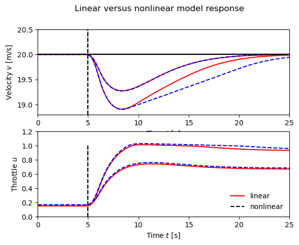
We apply the PI controller above to the case where the car is running with constant speed on a horizontal road and the system has stabilized so that the vehicle speed and the controller output are constant. The figure to the right shows what happens when the car encounters a hill with a slope of 4 degrees and a hill with a slope of 6 degrees at time Failed to parse (MathML with SVG or PNG fallback (recommended for modern browsers and accessibility tools): Invalid response ("Math extension cannot connect to Restbase.") from server "https://en.wikipedia.org/api/rest_v1/":): {\displaystyle t =\,}
5 seconds. The results for the nonlinear model are solid curves and those for the linear model are dashed curves. The differences between the curves are very small (especially for Failed to parse (MathML with SVG or PNG fallback (recommended for modern browsers and accessibility tools): Invalid response ("Math extension cannot connect to Restbase.") from server "https://en.wikipedia.org/api/rest_v1/":): {\displaystyle \theta =\,}
4 degrees), and control design based on the linearized model is thus validated.
Python code
Linearized dynamics
# Find the equilibrium point for the system
Xeq, Ueq = ct.find_eqpt(
vehicle, [vref[0]], [0, gear[0], theta0[0]], y0=[vref[0]], iu=[1, 2])
print("Xeq = ", Xeq)
print("Ueq = ", Ueq)
# Compute the linearized system at the eq pt
vehlin = ct.linearize(vehicle, Xeq, [Ueq[0], gear[0], 0, name='vehlin', copy=True])
# Create a closed loop controller for the linear system
cruise_lin = ct.InterconnectedSystem(
(vehlin, control_tf), name='cruise_linearized',
connections = [('control.u', '-vehlin'), ('vehlin.u', 'control.y')],
inplist = ('control.u', 'vehlin.gear', 'vehlin.theta'),
inputs = ('vref', 'gear', 'theta'),
outlist = ('vehlin.v', 'vehlin.u'), outputs = ('v', 'u'))
Simulations
# Linear response
t, y = ct.input_output_response(cruise_lin, T, [vref, gear, theta_hill], X0)
subplots = cruise_plot(cruise_tf, t, y, t_hill=5, linetype='b-')
# Nonlinear response
t, y = ct.input_output_response(cruise_tf, T, [vref, gear, theta_hill], X0)
cruise_plot(cruise_tf, t, y, t_hill=5, subplots=subplots, linetype='r-')
State Space Control
Further Reading

- How Stuff Works: cruise control
- Wikipedia: cruise control