Difference between revisions of "Figure 5.12: Stability analysis for a tanker"
Jump to navigation
Jump to search
(Created page with "{{Figure |Chapter=Dynamic Behavior |Figure number=5.12 |Sort key=512 |Figure title=Stability analysis for a tanker |GitHub URL=https://github.com/murrayrm/fbs2e-python/blob/ma...") |
|||
| (2 intermediate revisions by the same user not shown) | |||
| Line 5: | Line 5: | ||
|Figure title=Stability analysis for a tanker | |Figure title=Stability analysis for a tanker | ||
|GitHub URL=https://github.com/murrayrm/fbs2e-python/blob/main/example-5.8-tanker_stabilty.py | |GitHub URL=https://github.com/murrayrm/fbs2e-python/blob/main/example-5.8-tanker_stabilty.py | ||
| − | |Requires= | + | |Requires= |
}} | }} | ||
| + | [[Image:figure-5-12-tanker_stability.png]] | ||
| + | |||
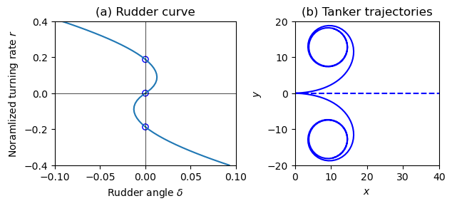
'''Figure 5.12''': Stability analysis for a tanker. The rudder characteristics are shown in (a), where the equilibrium points are marked by circles, and the tanker trajectories are shown in (b). | '''Figure 5.12''': Stability analysis for a tanker. The rudder characteristics are shown in (a), where the equilibrium points are marked by circles, and the tanker trajectories are shown in (b). | ||
| Line 108: | Line 110: | ||
# Save the figure | # Save the figure | ||
| − | plt.savefig("figure-5. | + | plt.savefig("figure-5.12-tanker_stability.png", bbox_inches='tight') |
</nowiki> | </nowiki> | ||
Latest revision as of 03:22, 17 November 2024
| Chapter | Dynamic Behavior |
|---|---|
| Figure number | 5.12 |
| Figure title | Stability analysis for a tanker |
| GitHub URL | https://github.com/murrayrm/fbs2e-python/blob/main/example-5.8-tanker stabilty.py |
| Requires | python-control, |
Figure 5.12: Stability analysis for a tanker. The rudder characteristics are shown in (a), where the equilibrium points are marked by circles, and the tanker trajectories are shown in (b).
# example-5.8-tanker_stability.py - Stability of a tanker
# RMM, 29 Aug 2021
#
# Figure 3.15: Stability analysis for a tanker. The rudder characteristics
# are shown in (a), where the equilibrium points are marked by circles, and
# the tanker trajec- tories are shown in (b).

import control as ct
import numpy as np
import matplotlib.pyplot as plt
ct.use_fbs_defaults()

#
# System dynamics
#

def tanker_dynamics(
        t, x, u, a1=-0.6, a2=-0.3, a3=-5, a4=-2, alpha=-2, b1=0.1, b2=-0.8):
    v, r = x[0], x[1]           # velocity and turning rate
    delta = u[0]                # rudder angle

    return [
        a1 * v + a2 * r + alpha * v * abs(v) + b1 * delta,
        a3 * v + a4 * r + b2 * delta
    ]
tanker_model = ct.nlsys(
    tanker_dynamics, None, inputs='delta', states=['v', 'r'])
print(tanker_model)


# Set up the plotting grid to match the layout in the book
fig = plt.figure(constrained_layout=True)
gs = fig.add_gridspec(2, 2)

#
# (a) Rudder curve
#
ax = fig.add_subplot(gs[0, 0])  # first row, first column

# Compute the input for each turning rate
rvec = np.linspace(-0.4, 0.4, 50)
delta_list = []
for r in rvec:
    # Solve for the different equilibrium solutions
    eqpt = ct.find_operating_point(
        tanker_model, [0, 0], 0,
        y0=[0, r], iy=[1],      # Look for the desired turning rate
    )
    delta_list.append(eqpt.inputs[0])
dvec = np.array(delta_list)
ax.plot(dvec, rvec)

# Add the equilibrium points at zero
for x0 in [[0.1, 0.1], [0, 0], [-0.1, -0.1]]:
    eqpt = ct.find_operating_point(tanker_model, x0, 0)
    ax.scatter(
        eqpt.inputs[0], eqpt.outputs[1], facecolors='none', edgecolors='b')

# Add labels and axis lines
ax.set_title("(a) Rudder curve")
ax.set_xlabel(r"Rudder angle $\delta$")
ax.set_ylabel(r"Noramlized turning rate $r$")
ax.plot([-0.1, 0.1], [0, 0], 'k', linewidth=0.5)
ax.plot([0, 0], [-0.4, 0.4], 'k', linewidth=0.5)
ax.axis([-0.1, 0.1, -0.4, 0.4])

#
# (b) Tanker trajectories
#
from math import sin, cos
ax = fig.add_subplot(gs[0, 1])  # first row, second column

# Create a full tanker model, including position and orientation
def full_tanker_dynamics(t, x, u, **params):
    vdot, rdot = tanker_dynamics(t, x[3:], u, **params)
    theta, v, r = x[2], x[3], x[4]
    return [
        cos(theta) + v * sin(theta), -sin(theta) + v * cos(theta),
        r, vdot, rdot]
full_tanker_model = ct.nlsys(
    full_tanker_dynamics, None, inputs='delta',
    states=['x', 'y', 'theta', 'v', 'r'])

# Create simulations and plot them
timepts = np.linspace(0, 100, 100)
for r0, linestyle in zip([0.1, 0, -0.1], ['b-', 'b--', 'b-']):
    response = ct.input_output_response(
        full_tanker_model, timepts, 0, [0, 0, 0, 0, r0])
    ax.plot(response.outputs[0], response.outputs[1], linestyle)

# Add labels and axis lines
ax.set_title("(b) Tanker trajectories")
ax.set_xlabel("$x$")
ax.set_ylabel("$y$")
ax.axis('scaled')
ax.axis([0, 40, -20, 20])

# Save the figure
plt.savefig("figure-5.12-tanker_stability.png", bbox_inches='tight')
