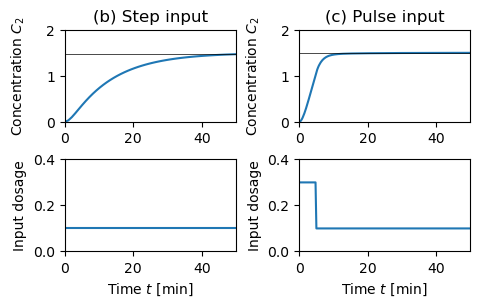
Figure 6.10: Response of a compartment model to a constant drug infusion

Chapter	Linear Systems
Figure number	6.10
Figure title	Response of a compartment model to a constant drug infusion
GitHub URL	https://github.com/murrayrm/fbs2e-python/blob/main/example-6.10-compartment response.py
Requires	python-control

Figure 6.10: Response of a compartment model to a constant drug infusion. A simple diagram of the system is shown in (a). The step response (b) shows the rate of concentration buildup in compartment 2. In (c) a pulse of initial concentration is used to speed up the response.

# example-6.7-compartment_response.py - Compartment model response
# RMM, 24 Nov 2024
#
# Figure 6.10: Response of a compartment model to a constant drug
# infusion. A simple diagram of the system is shown in (a). The step
# response (b) shows the rate of concentration buildup in compartment 2. In
# (c) a pulse of initial concentration is used to speed up the response.

import control as ct
import numpy as np
import matplotlib.pyplot as plt
ct.use_fbs_defaults()

#
# System dynamics
#

# Parameter settings for the model
k0 = 0.1
k1 = 0.1
k2 = 0.5
b0 = 1.5

# Compartment model definition
Ada = np.array([[-k0 - k1, k1], [k2, -k2]])
Bda = np.array([[b0], [0]])
Cda = np.array([[0, 1]])
compartment = ct.ss(Ada, Bda, Cda, 0);

# Set up the plotting grid to match the layout in the book
fig = plt.figure(constrained_layout=True)
gs = fig.add_gridspec(4, 3)

#
# (a) Step input
#

timepts = np.linspace(0, 50)
input = np.ones(timepts.size) * 0.1
response = ct.forced_response(compartment, timepts, input)

ax = fig.add_subplot(gs[0, 1])
ax.set_title("(b) Step input")

ax.plot(response.time, response.outputs)
ax.axhline(response.outputs[-1], color='k', linewidth=0.5)
ax.set_ylabel("Concentration $C_2$")
ax.axis('tight')
ax.axis([0, 50, 0, 2])

ax = fig.add_subplot(gs[1, 1])
ax.plot(response.time, response.inputs)
ax.set_xlabel("Time $t$ [min]")
ax.set_ylabel("Input dosage")
ax.axis('tight')
ax.axis([0, 50, 0, 0.4])

#
# (b) Pulse input
#

timepts = np.linspace(0, 50, 200)
input = np.ones(timepts.size) * 0.1
input[:20] = 0.3                # Increase value for first 5 seconds
response = ct.forced_response(compartment, timepts, input)

ax = fig.add_subplot(gs[0, 2])
ax.set_title("(c) Pulse input")

ax.plot(response.time, response.outputs)
ax.axhline(response.outputs[-1], color='k', linewidth=0.5)
ax.set_ylabel("Concentration $C_2$")
ax.axis('tight')
ax.axis([0, 50, 0, 2])

ax = fig.add_subplot(gs[1, 2])
ax.plot(response.time, response.inputs)
ax.set_xlabel("Time $t$ [min]")
ax.set_ylabel("Input dosage")
ax.axis('tight')
ax.axis([0, 50, 0, 0.4])

# Save the figure
fig.align_ylabels()
plt.savefig("figure-6.10-compartment_response.png", bbox_inches='tight')