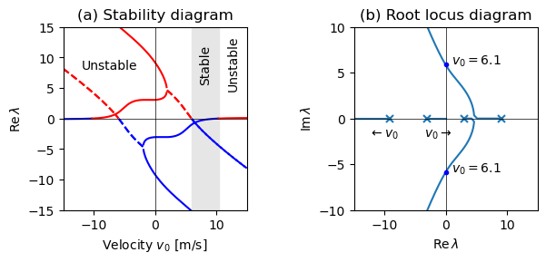
Figure 5.19: Stability plots for a bicycle moving at constant velocity

Chapter	Dynamic Behavior
Figure number	5.19
Figure title	Stability plots for a bicycle moving at constant velocity
GitHub URL	https://github.com/murrayrm/fbs2e-python/blob/main/example-5.17-bicycle stability.py
Requires	python-control, bicycle.py

Figure 5.19: Stability plots for a bicycle moving at constant velocity. The plot in (a) shows the real part of the system eigenvalues as a function of the bicycle velocity $v_{0}$. The system is stable when all eigenvalues have negative real part (shaded region). The plot in (b) shows the locus of eigenvalues on the complex plane as the velocity $v$ is varied and gives a different view of the stability of the system. This type of plot is called a root locus diagram.

Note: The line styles used in this plot are slightly different than in the book. Solid lines are used for real-valued eigenvalues and dashed lines are used for the real part of complex-valued eigenvalues.

# example-5.17-bicycle_stability.py - Root locus diagram for a bicycle model
# RMM, 24 Nov 2024
#
# Figure 5.19: Stability plots for a bicycle moving at constant
# velocity. The plot in (a) shows the real part of the system eigenvalues
# as a function of the bicycle velocity v0. The system is stable when all
# eigenvalues have negative real part (shaded region). The plot in (b)
# shows the locus of eigenvalues on the complex plane as the velocity v is
# varied and gives a different view of the stability of the system. This
# type of plot is called a root locus diagram.
#
# Notes:
#
# 1. The line styles used in this plot are slightly different than in the
#    book.  Solid lines are used for real-valued eigenvalues and dashed
#    lines are used for the real part of complex-valued eigenvalues.
#
# 2. This code relies on features on python-control-0.10.2, which is
#    currently under development.

import control as ct
import numpy as np
import matplotlib.pyplot as plt
from math import isclose
ct.use_fbs_defaults()

#
# System dynamics
#

from bicycle import whipple_A

# Set up the plotting grid to match the layout in the book
fig = plt.figure(constrained_layout=True)
gs = fig.add_gridspec(2, 2)

#
# (a) Stability diagram
#

ax = fig.add_subplot(gs[0, 0])  # first row, first column
ax.set_title("(a) Stability diagram")

# Compute the eigenvalues as a function of velocity
v0_vals = np.linspace(-15, 15, 500)
eig_vals = []
for v0 in v0_vals:
    A = whipple_A(v0)
    eig_vals.append(np.sort(np.linalg.eig(A).eigenvalues))

# Initialize lists to categorize eigenvalues
eigs_real_stable = []
eigs_complex_stable = []
eigs_real_unstable = []
eigs_complex_unstable = []

# Keep track of region in which all eigenvalues are stable
stable_beg = stable_end = None

# Process each set of eigenvalues
for i, eig_set in enumerate(eig_vals):
    # Create arrays filled with NaN for each category
    real_stable = np.full(eig_set.shape, np.nan)
    complex_stable = np.full(eig_set.shape, np.nan)
    real_unstable = np.full(eig_set.shape, np.nan)
    complex_unstable = np.full(eig_set.shape, np.nan)
    
    # Classify eigenvalues
    for j, eig in enumerate(eig_set):
        if isclose(eig.imag, 0):  # Real eigenvalue
            if eig.real < 0:
                real_stable[j] = eig.real
            else:
                real_unstable[j] = eig.real
        else:  # Complex eigenvalue
            if eig.real < 0:
                complex_stable[j] = eig.real
            else:
                complex_unstable[j] = eig.real

    # Append categorized arrays to respective lists
    eigs_real_stable.append(real_stable)
    eigs_complex_stable.append(complex_stable)
    eigs_real_unstable.append(real_unstable)
    eigs_complex_unstable.append(complex_unstable)

    # Look for regions where everything is stable
    if stable_beg is None and all(eig_set.real < 0):
        stable_beg = i
    elif stable_beg and stable_end is None and any(eig_set.real > 0):
        stable_end = i

# Plot the stability diagram
ax.plot(v0_vals, eigs_real_stable, 'b-')
ax.plot(v0_vals, eigs_real_unstable, 'r-')
ax.plot(v0_vals, eigs_complex_stable, 'b--')
ax.plot(v0_vals, eigs_complex_unstable, 'r--')

# Add in the coordinate axes
ax.axhline(color='k', linewidth=0.5)
ax.axvline(color='k', linewidth=0.5)

# Label and shade stable and unstable regions
ax.text(-12, 8, "Unstable")
ax.fill_betweenx(
    [-15, 15], [v0_vals[stable_beg], v0_vals[stable_beg]],
    [v0_vals[stable_end], v0_vals[stable_end]], color='0.9')
ax.text(7.2, 6, "Stable", rotation=90)
ax.text(11.7, 5, "Unstable", rotation=90)

# Label the axes
ax.set_xlabel(r"Velocity $v_0$ [m/s]")
ax.set_ylabel(r"$\text{Re}\,\lambda$")
ax.axis('scaled')
ax.axis([-15, 15, -15, 15])

#
# (b) Root locus diagram
#

ax = fig.add_subplot(gs[0, 1])  # first row, second column
ax.set_title("(b) Root locus diagram")

# Generate the root locus diagram via the root_locus_plot functionality
pos_idx = np.argmax(v0_vals >= 0)
poles = eig_vals[pos_idx]
loci = np.array(eig_vals[pos_idx:])
rl_map = ct.PoleZeroData(poles, [], v0_vals[pos_idx:], loci)
rl_map.plot(ax=ax)

# Add in the coordinate axes
ax.axhline(color='k', linewidth=0.5)
ax.axvline(color='k', linewidth=0.5)

# Label the real axes of the plot
ax.text(-12.5, -2, r"$\leftarrow v_0$")
ax.text(-3.5, -2, r"$v_0 \rightarrow$")

# Label the crossover points
xo_idx = np.argmax(rl_map.loci[:, 3].real < 0)
ax.plot(0, rl_map.loci[xo_idx, 2].imag, 'bo', markersize=3)
ax.plot(0, rl_map.loci[xo_idx, 3].imag, 'bo', markersize=3)
ax.text(1, rl_map.loci[xo_idx, 2].imag, r"$v_0 = 6.1$")
ax.text(1, rl_map.loci[xo_idx, 3].imag, r"$v_0 = 6.1$")

# Label the axes
ax.set_xlabel(r"$\text{Re}\,\lambda$")
ax.set_ylabel(r"$\text{Im}\,\lambda$")
ax.set_box_aspect(1)
ax.axis([-15, 15, -10, 10])

# Save the figure
plt.savefig("figure-5.19-bicycle_stability.png", bbox_inches='tight')