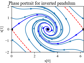
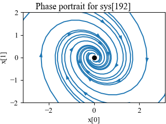
Figure 5.11: Comparison between phase portraits for a nonlinear system and its linearization

Chapter	Dynamic Behavior
Figure number	5.11
Figure title	Comparison between phase portraits for a nonlinear system and its linearization
GitHub URL	https://github.com/murrayrm/fbs2e-python/blob/main/figure-5.11-invpend linearized.py
Requires	python-control

 

Figure 5.11: Comparison between the phase portraits for the full nonlinear system (a) and its linear approximation around the origin (b). Notice that near the equilibrium point at the center of the plots, the phase portraits (and hence the dynamics) are almost identical.

# invepend_linearized.py - nonlinear vs linear inverted pendulum dynamics
# RMM, 7 Apr 2024

import matplotlib.pyplot as plt
import numpy as np
from math import pi
import control as ct
import fbs                      # FBS plotting customizations

def invpend_update(t, x, u, params):
    m, l, b, g = params['m'], params['l'], params['b'], params['g']
    return [x[1], -b/m * x[1] + (g * l / m) * np.sin(x[0])]
invpend = ct.nlsys(
    invpend_update, states=2, inputs=0, name='inverted pendulum',
    params={'m': 1, 'l': 1, 'b': 0.5, 'g': 1})

fbs.figure()
ct.phase_plane_plot(
    invpend, [0, 2*pi, -2, 2], 6, gridspec=[6, 5],
    plot_separatrices={'timedata': 20, 'arrows': 4})
fbs.savefig('figure-5.10-invpend_linearized-nl.png')

# Create a linearized model
linsys = invpend.linearize([pi, 0], 0)

fbs.figure()
ct.phase_plane_plot(
    linsys, [-pi, pi, -2, 2], 10, gridspec=[5, 2],
    plot_separatrices={'timedata': 20, 'arrows': 4})
fbs.savefig('figure-5.10-invpend_linearized-ln.png')