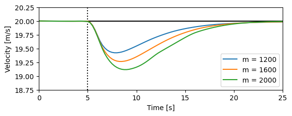
Figure 1.11: A feedback system for controlling the velocity of a vehicle

Chapter	Introduction
Figure number	1.11
Figure title	A feedback system for controlling the velocity of a vehicle
GitHub URL	https://github.com/murrayrm/fbs2e-python/blob/main/figure-1.11-cruise robustness.py
Requires	python-control, cruise.py

Figure 1.11: A feedback system for controlling the velocity of a vehicle. In the block diagram on the left, the velocity of the vehicle is measured and compared to the desired velocity within the “Compute” block. Based on the difference in the actual and desired velocities, the throttle (or brake) is used to modify the force applied to the vehicle by the engine, drivetrain, and wheels. The figure on the right shows how the velocity changes when the car travels on a horizontal road and the slope of the road changes to a constant uphill slope. The three different curves correspond to differing masses of the vehicle, between 1200 and 2000 kg, demonstrating that feedback can indeed compensate for the changing slope and that the closed loop system is robust to a large change in the vehicle characteristics.

# figure-1.11-cruise_robustness.py - Cruise control w/ range of vehicle masses
# RMM, 20 Jun 2021
# 
# This script generates the response of the system to a 4 deg hill with
# different vehicles masses.  The figure shows how the velocity changes when
# the car travels on a horizontal road and the slope of the road changes to
# a constant uphill slope. The three different curves correspond to
# differing masses of the vehicle, between 1200 and 2000 kg, demonstrating
# that feedback can indeed compensate for the changing slope and that the
# closed loop system is robust to a large change in the vehicle
# characteristics.

# Package import
import numpy as np
import matplotlib.pyplot as plt
import control as ct
import cruise                   # vehicle dynamics, PI controller

# Define the time and input vectors
T = np.linspace(0, 25, 101)
vref = 20 * np.ones(T.shape)
gear = 4 * np.ones(T.shape)
theta0 = np.zeros(T.shape)

# Now simulate the effect of a hill at t = 5 seconds
theta_hill = np.array([
    0 if t <= 5 else
    4./180. * np.pi * (t-5) if t <= 6 else
    4./180. * np.pi for t in T])

# Create the plot and add a line at the reference speed
plt.subplot(2, 1, 1)
plt.axis([0, T[-1], 18.75, 20.25])
plt.plot([T[0], T[-1]], [vref[0], vref[-1]], 'k-')      # reference velocity
plt.plot([5, 5], [18.75, 20.25], 'k:')                  # disturbance start

masses = [1200, 1600, 2000]
for i, m in enumerate(masses):
    # Compute the equilibrium state for the system
    X0, U0 = ct.find_eqpt(
        cruise.cruise_PI,
        [vref[0], 0],
        [vref[0], gear[0], theta0[0]], 
        iu=[1, 2], y0=[vref[0], 0], iy=[0], params={'m': m})

    # Simulate the effect of a hill
    t, y = ct.input_output_response(
        cruise.cruise_PI, T,
        [vref, gear, theta_hill],
        X0, params={'m':m})

    # Plot the response for this mass
    plt.plot(t, y[cruise.cruise_PI.find_output('v')], label='m = %d' % m)

# Add labels and legend to the plot
plt.xlabel('Time [s]')
plt.ylabel('Velocity [m/s]')
plt.legend()