Exercise: Exploring the dynamics of a rolling mill

Chapter	Introduction
Exercise number
Author(s)	Lars Cremean
Created	2002/09/01

Download the file “rolling_mill.py", which contains a model of a rolling mill, a machine used to create material (paper, steel, etc) of a given thickness (described in a bit more detail below).

(a) Run the simulation with default parameters and create a plot of the output thickness versus time.

(b) While keeping the proportional gain fixed at its default value, vary the integral gain from zero to twice the default simulation value. Give the value for which the system begins to go unstable. Plot the settling time as a function of $K_{\text{i}}$ for the stable cases.

(c) While keeping fixed at its default value, vary from zero to twice the default simulation value. Give the value for which the system begins to go unstable. Plot the settling time as a function of for the stable cases.

All plots should included a title, labeled axes (with units), and reasonable axis limits.

Note: It is not necessary for you to understand the dynamics of the process and control law at this point.

Rolling mill dynamics

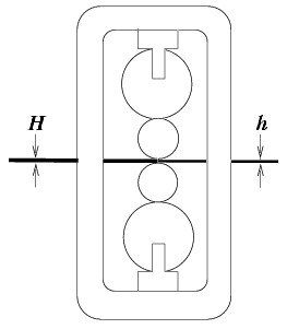
The rolling mill example is a simplified model of a steel rolling mill. The control problem is to control the exit thickness of a sheet of steel that is fed between two rollers, as shown below The exit thickness h of the steel is related to the gap between the rollers, which depends on the unloaded position of backup rollers (also called the screw position), and the input thickness . The force on the rollers is reasonably modeled by

</math>

F = M (h -s)

</math>

as well as

</math>

F = W (H - h)

</math>

where $H$ and $W$ are constants.

Combining these two gives

$h(M+W)=Ms+WH$

Measurement and actuator dynamics are modeled with time delays of 1 second and 0.01 seconds, respectively. A proportional-integral control law is incorporated into the model whose job is to try and regulate the output thickness to the desired thickness.

Notes

• The output thickness for each run is saved to the MATLAB workspace as a structure called "rollmill". You can access the elements of a structure using a period (.), e.g. rollmill.signals...
• The settling time is the time it takes for the system error to settle to within the desired thickness plus or minus 5%. Any method of finding these values to produce your plots is acceptable, but you may like to investigate the MATLAB "find" command.
• Include at least ten values in each of your settling time versus plots.
• Include a title, axis labels (with units), and reasonable axis limits on all plots. See MATLAB commands "title", "axis", "ylabel" and "xlabel".