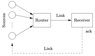
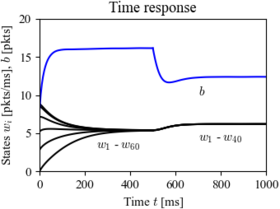
Figure 4.13: Internet congestion control for N identical sources across a single link

Chapter	Examples
Figure number	4.13
Figure title	Internet congestion control for N identical sources across a single link
GitHub URL	https://github.com/murrayrm/fbs2e-python/blob/main/figure-4.13-congctrl tcpsim.py
Requires	python-control, congctrl.py

  

Figure 4.13: Internet congestion control for N identical sources across a single link. As shown on the left, multiple sources attempt to communicate through a router across a single link. An “ack” packet sent by the receiver acknowledges that the message was received; otherwise the message packet is resent and the sending rate is slowed down at the source. The simulation on the right is for 60 sources starting at random rates (window sizes), with 20 sources dropping out at t = 500 ms. The buffer size is shown at the top, and the individual source rates for 6 of the sources are shown at the bottom.

# congctrl_tcpsim.m - congestion control simulation
# RMM, 9 Sep 2006 (from MATLAB)

import matplotlib.pyplot as plt
import numpy as np
import random
import control as ct
import congctrl
import fbs                      # FBS plotting customizations

# Create an I/O system for simulation
M = 6                           # simulate 6 aggregated sources
N = 60                          # modeling 60 independent sources
congctrl_sys = congctrl.create_iosystem(M, N=N)

# Find the equilibrium point
xeq, ueq = ct.find_eqpt(congctrl_sys, np.ones(M+1), 0)
weq, beq = xeq[0], xeq[-1]              # first N states are identical

# Compute a perturbation for the initial condition
random.seed(6)                          # for repeatability
w0 = np.array([
    weq + 2 * (random.random() - 0.5) * weq for i in range(M)])
b0 = beq/2

# Run a simulation
tvec = np.linspace(0, 500, 100)
resp = ct.input_output_response(
    congctrl_sys, tvec, U=0, X0=[w0, b0])

# Plot the results
# Set up a figure for plotting the results
fbs.figure('mlh')

for i in range(M):
    plt.plot(resp.time, resp.states[i], 'k')
plt.plot(resp.time, resp.states[-1] / 20, 'b')

# Now change the number of sources and rerun from the old initial condition
M = 4                           # simulate 4 aggregated sources
N = 40                          # modeling 40 independent sources
congctrl_pert = congctrl.create_iosystem(M, N=N)

# Run a simulation starting from where we left off
tvec = np.linspace(500, 1000, 100)
pert = ct.input_output_response(
    congctrl_pert, tvec, U=0, X0=[resp.states[0:4, -1], resp.states[-1, -1]])

# Plot the results
for i in range(M):
    plt.plot(pert.time, pert.states[i], 'k')
plt.plot(pert.time, pert.states[-1] / 20, 'b')

# Label the plots and make them pretty
plt.axis([0, 1000, 0, 20])
plt.xlabel("Time $t$ [ms]")
plt.ylabel("States $w_i$ [pkts/ms], $b$ [pkts]")
plt.title("Time response")
plt.text(250, 3, "$w_1$ - $w_{60}$")
plt.text(700, 4, "$w_1$ - $w_{40}$")
plt.text(700, 10, "$b$")

# Save the figure
fbs.savefig('figure-4.13-congctrl_tcpsim.png')          # PNG for web