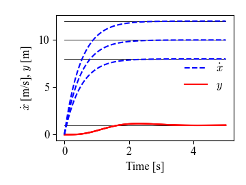
Figure 8.13: Vehicle steering using gain scheduling
Jump to navigation
Jump to search
| Chapter | Output Feedback |
|---|---|
| Figure number | 8.13 |
| Figure title | Vehicle steering using gain scheduling |
| GitHub URL | https://github.com/murrayrm/fbs2e-python/blob/main/example-8.10-steering gainsched.py |
| Requires | python-control, fbs.py |
Figure 8.13: Vehicle steering using gain scheduling. (a) Vehicle configuration consists of the x, y position of the vehicle, its angle with respect to the road, and the steering wheel angle. (b) Step responses for the vehicle lateral position (solid) and forward velocity (dashed). Gain scheduling is used to set the feedback controller gains for the different forward velocities.
# example-8.10-steering_gainsched.py - gain scheduling for vehicle steering
# RMM, 8 May 2019 (updated 6 Oct 2021)

import numpy as np
import control as ct
from cmath import sqrt
import matplotlib.pyplot as mpl

#
# Vehicle steering dynamics
#
# The vehicle dynamics are given by a simple bicycle model.  We take the state
# of the system as (x, y, theta) where (x, y) is the position of the vehicle
# in the plane and theta is the angle of the vehicle with respect to
# horizontal.  The vehicle input is given by (v, phi) where v is the forward
# velocity of the vehicle and phi is the angle of the steering wheel.  The
# model includes saturation of the vehicle steering angle.
#
# System state: x, y, theta
# System input: v, phi
# System output: x, y
# System parameters: wheelbase, maxsteer
#
def vehicle_update(t, x, u, params):
    # Get the parameters for the model
    l = params.get('wheelbase', 3.)         # vehicle wheelbase
    phimax = params.get('maxsteer', 0.5)    # max steering angle (rad)

    # Saturate the steering input
    phi = np.clip(u[1], -phimax, phimax)

    # Return the derivative of the state
    return np.array([
        np.cos(x[2]) * u[0],            # xdot = cos(theta) v
        np.sin(x[2]) * u[0],            # ydot = sin(theta) v
        (u[0] / l) * np.tan(phi)        # thdot = v/l tan(phi)
    ])

def vehicle_output(t, x, u, params):
    return x                            # return x, y, theta (full state)

# Define the vehicle steering dynamics as an input/output system
vehicle = ct.NonlinearIOSystem(
    vehicle_update, vehicle_output, states=3, name='vehicle',
    inputs=('v', 'phi'),
    outputs=('x', 'y', 'theta'))

#
# Gain scheduled controller
#
# For this system we use a simple schedule on the forward vehicle velocity and
# place the poles of the system at fixed values.  The controller takes the
# current and desired vehicle position and orientation plus the velocity
# velocity as inputs, and returns the velocity and steering commands.
#
# System state: none
# System input: x, y, theta, xd, yd, thetad, vd, phid
# System output: v, phi
# System parameters: longpole, latomega_c, latzeta_c
#
def control_output(t, x, u, params):
    # Get the controller parameters
    longpole = params.get('longpole', -2.)
    latomega_c = params.get('latomega_c', 2)
    latzeta_c = params.get('latzeta_c', 0.5)
    l = params.get('wheelbase', 3)

    # Extract the system inputs and compute the errors
    x, y, theta, xd, yd, thetad, vd, phid = u
    ex, ey, etheta = x - xd, y - yd, theta - thetad

    # Determine the controller gains
    lambda1 = -longpole
    a1 = 2 * latzeta_c * latomega_c
    a2 = latomega_c**2

    # Compute and return the control law
    v = -lambda1 * ex           # leave off feedforward to generate transient
    if vd != 0:
        phi = phid - ((a2 * l) / vd**2) * ey - ((a1 * l) / vd) * etheta
    else:
        # We aren't moving, so don't turn the steering wheel
        phi = phid

    return  np.array([v, phi])

# Define the controller as an input/output system
controller = ct.NonlinearIOSystem(
    None, control_output, name='controller',            # static system
    inputs=('x', 'y', 'theta', 'xd', 'yd', 'thetad',    # system inputs
            'vd', 'phid'),
    outputs=('v', 'phi')                                # system outputs
)

#
# Reference trajectory subsystem
#
# The reference trajectory block generates a simple trajectory for the system
# given the desired speed (vref) and lateral position (yref).  The trajectory
# consists of a straight line of the form (vref * t, yref, 0) with nominal
# input (vref, 0).
#
# System state: none
# System input: vref, yref
# System output: xd, yd, thetad, vd, phid
# System parameters: none
#
def trajgen_output(t, x, u, params):
    vref, yref = u
    return np.array([vref * t, yref, 0, vref, 0])

# Define the trajectory generator as an input/output system
trajgen = ct.NonlinearIOSystem(
    None, trajgen_output, name='trajgen',
    inputs=('vref', 'yref'),
    outputs=('xd', 'yd', 'thetad', 'vd', 'phid'))

#
# System construction
#
# The input to the full closed loop system is the desired lateral position and
# the desired forward velocity.  The output for the system is taken as the
# full vehicle state plus the velocity of the vehicle.
#
# We construct the system using the InterconnectedSystem constructor and using
# signal labels to keep track of everything.

steering = ct.interconnect(
    # List of subsystems
    (trajgen, controller, vehicle), name='steering',

    # System inputs
    inplist=['trajgen.vref', 'trajgen.yref'],
    inputs=['yref', 'vref'],

    #  System outputs
    outlist=['vehicle.x', 'vehicle.y', 'vehicle.theta', 'controller.v',
             'controller.phi'],
    outputs=['x', 'y', 'theta', 'v', 'phi']
)

# Set up the simulation conditions
yref = 1
T = np.linspace(0, 5, 100)

# Set up a figure for plotting the results
mpl.figure(figsize=[3.2, 2.4], tight_layout=True)

# Plot the reference trajectory for the y position
mpl.plot([0, 5], [yref, yref], 'k--')

# Find the signals we want to plot
y_index = steering.find_output('y')
v_index = steering.find_output('v')

# Do an iteration through different speeds
for vref in [8, 10, 12]:
    # Simulate the closed loop controller response
    tout, yout = ct.input_output_response(
        steering, T, [vref * np.ones(len(T)), yref * np.ones(len(T))])

    # Plot the reference speed
    mpl.plot([0, 5], [vref, vref], 'k--')

    # Plot the system output
    y_line, = mpl.plot(tout, yout[y_index, :], 'r')  # lateral position
    v_line, = mpl.plot(tout, yout[v_index, :], 'b')  # vehicle velocity

# Add axis labels
mpl.xlabel('Time [s]')
mpl.ylabel('$x$ vel [m/s], $y$ pos [m]')
mpl.legend((v_line, y_line), ('$v$', '$y$'), loc='center right', frameon=False)

# Save the figure
mpl.savefig('figure-8.13-steering_gainsched.png')
