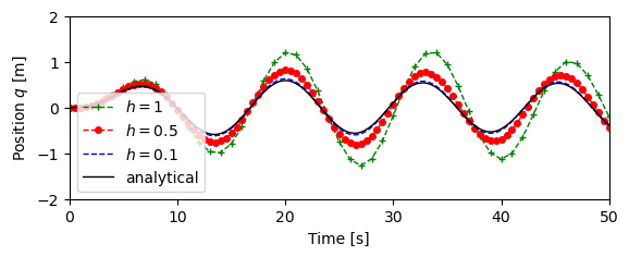
Figure 3.11: Simulation of the forced spring–mass system with different simulation time constants

Chapter	System Modeling
Figure number	11
Figure title	Simulation of the forced spring–mass system with different simulation time constants
GitHub URL	https://github.com/murrayrm/fbs2e-python/blob/main/figure-3.11-spring mass simulation.py
Requires	python-control

Figure 3.11: Simulation of the forced spring–mass system with different simulation time constants. The solid line represents the analytical solution. The dashed lines represent the approximate solution via the method of Euler integration, using decreasing step sizes.

# figure-3.11-spring_mass_simulation.py - forced spring–mass simulation approx
# RMM, 28 Aug 2021
#
# Figure 3.11: Simulation of the forced spring–mass system with
# different simulation time constants. The solid line represents the
# analytical solution. The dashed lines represent the approximate
# solution via the method of Euler integration, using decreasing step
# sizes.
#

import numpy as np
import matplotlib.pyplot as plt
import control as ct
ct.use_fbs_defaults()

# Parameters defining the system
m = 250                         # system mass
k = 40                          # spring constant
b = 60                          # damping constant

# System matrices
A = [[0, 1], [-k/m, -b/m]]
B = [0, 1/m]
C = [1, 0]
sys = ct.ss(A, B, C, 0)

#
# Discrete time simulation
#
# This section explores what happens when we discretize the ODE
# and convert it to a discrete time simulation.
#
Af = 20                         # forcing amplitude
omega = 0.5                     # forcing frequency

# Sinusoidal forcing function
t = np.linspace(0, 100, 1000)
u = Af * np.sin(omega * t)

# Simulate the system using standard MATLAB routines
response = ct.forced_response(sys, t, u)
ts, ys = response.time, response.outputs

#
# Now generate some simulations manually
#

# Time increments for discrete approximations
hvec = [1, 0.5, 0.1]                # h must be a multiple of 0.1
max_len = int(t[-1] / min(hvec))    # maximum number of time steps

# Create arrays for storing results
td = np.zeros((len(hvec), max_len)) # discrete time instants
yd = np.zeros((len(hvec), max_len)) # output at discrete time instants

# Discrete time simulations
maxi = []                           # list to store maximum index
for iter, h in enumerate(hvec):
    maxi.append(round(t[-1] / h))   # save maximum index for this h
    x = np.zeros((2, maxi[-1] + 1)) # create an array to store the state

    # Compute the discrete time Euler approximation of the dynamics
    for i in range(maxi[-1]):
        offset = int(h/0.1 * i)     # input offset
        x[:, i+1] = x[:, i] + h * (sys.A @ x[:, i] + (sys.B * u[offset])[:, 0])
        td[iter, i] = (i-1) * h
        yd[iter, i] = sys.C @ x[:, i]

# Plot the results
plt.subplot(2, 1, 1)

simh = plt.plot(
    td[0, 0:maxi[0]], yd[0, 0:maxi[0]], 'g+--',
    td[1, 0:maxi[1]], yd[1, 0:maxi[1]], 'ro--',
    td[2, 0:maxi[2]], yd[2, 0:maxi[2]], 'b--',
    markersize=4, linewidth=1
)
analh = plt.plot(ts, ys, 'k-', linewidth=1)

plt.xlabel("Time [s]")
plt.ylabel("Position $q$ [m]")
plt.axis([0, 50, -2, 2])
plt.legend(["$h = %g$" % h for h in hvec] + ["analytical"]), 

# Save the figure
plt.savefig("figure-3.11-spring_mass_simulation.png", bbox_inches='tight')