Difference between revisions of "Figure 2.8: Step responses for a first-order, closed loop system with proportional and PI control"
Jump to navigation
Jump to search
(Created page with "{{Figure |Chapter=Feedback Principles |Figure number=2.8 |Figure title=Step responses for a first-order, closed loop system with proportional # control and PI control. |GitHub...") |
|||
| (8 intermediate revisions by the same user not shown) | |||
| Line 2: | Line 2: | ||
|Chapter=Feedback Principles | |Chapter=Feedback Principles | ||
|Figure number=2.8 | |Figure number=2.8 | ||
| + | |Sort key=208 | ||
|Figure title=Step responses for a first-order, closed loop system with proportional # control and PI control. | |Figure title=Step responses for a first-order, closed loop system with proportional # control and PI control. | ||
|GitHub URL=https://github.com/murrayrm/fbs2e-python/blob/main/figure-2.8-PI_step_responses.py | |GitHub URL=https://github.com/murrayrm/fbs2e-python/blob/main/figure-2.8-PI_step_responses.py | ||
| Line 7: | Line 8: | ||
[[Image:figure-2.8-PI_step_response.png]] | [[Image:figure-2.8-PI_step_response.png]] | ||
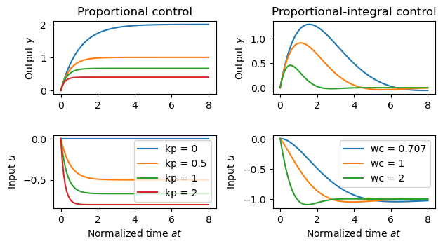
| − | '''Figure 2.8''': Step responses for a first-order, closed loop system with proportional control (a) and PI control (b). The process transfer function is | + | '''Figure 2.8''': Step responses for a first-order, closed loop system with proportional control (a) and PI control (b). The process transfer function is <math>P = 2/(s + 1)</math>. The controller gains for proportional control are <math>k_\text{p} =</math> 0, 0.5, 1, and 2. The PI controller is designed using equation (2.28) with <math>\zeta_\text{c} =</math> 0.707 and <math>\omega_\text{c} =</math> 0.707, 1, and 2, which gives the controller parameters <math>k_\text{p} =</math> 0, 0.207, and 0.914 and <math>k_\text{i} =</math> 0.25, 0.50, and 2. |
<nowiki> | <nowiki> | ||
| Line 96: | Line 97: | ||
pi_u_ax.legend() | pi_u_ax.legend() | ||
| − | # | + | # Overall figure labeling |
plt.tight_layout() | plt.tight_layout() | ||
</nowiki> | </nowiki> | ||
Latest revision as of 16:45, 28 May 2023
| Chapter | Feedback Principles |
|---|---|
| Figure number | 2.8 |
| Figure title | Step responses for a first-order, closed loop system with proportional # control and PI control. |
| GitHub URL | https://github.com/murrayrm/fbs2e-python/blob/main/figure-2.8-PI step responses.py |
| Requires | python-control |
Figure 2.8: Step responses for a first-order, closed loop system with proportional control (a) and PI control (b). The process transfer function is . The controller gains for proportional control are 0, 0.5, 1, and 2. The PI controller is designed using equation (2.28) with 0.707 and 0.707, 1, and 2, which gives the controller parameters 0, 0.207, and 0.914 and 0.25, 0.50, and 2.
# figure-2.8-PI_step_reesponses.py - step responses for P/PI controllers
# RMM, 21 Jun 2021
#
# Step responses for a first-order, closed loop system with proportional
# control and PI control. The process transfer function is P = 2/(s + 1).
# The controller gains for proportional control are k_p = 0, 0.5, 1, and
# 2. The PI controller is designed using equation (2.28) with zeta_c = 0.707
# and omega_c = 0.707, 1, and 2, which gives the controller parameters k_p =
# 0, 0.207, and 0.914 and k_i = 0.25, 0.50, and 2.
#

import numpy as np
import matplotlib.pyplot as plt
import control as ct

# Process model
b = 2; a = 1
P = ct.tf([b], [1, a])

# Set the simulation time vector
time = np.linspace(0, 8, 100)

#
# Proportional control
#

# Choose gains to use
kp_gains = [0, 0.5, 1, 2]

for kp in kp_gains:
    Gyv = ct.tf([b], [1, a + b*kp])
    Guv = ct.tf([-b*kp], [1, a + b*kp], dt=0)   # force kp=0 to be cts time

    t, y = ct.step_response(Gyv, time)
    t, u = ct.step_response(Guv, time)

    if 'p_y_ax' not in locals():
        p_y_ax = plt.subplot(3, 2, 1)
        plt.ylabel('Output $y$')
        plt.title('Proportional control')
    p_y_ax.plot(t, y)

    if 'p_u_ax' not in locals():
        p_u_ax = plt.subplot(3, 2, 3)
        plt.ylabel('Input $u$')
        plt.xlabel('Normalized time $at$')
    p_u_ax.plot(t, u, label="kp = %0.3g" % kp)

# Label proportional control curves
p_u_ax.legend()

#
# PI control
#

# Figure out frequency of critical damping
zeta = 0.707
wc = a / 2 / zeta

# Plot results for different resonate frequencies
wc_list = [wc, 1, 2]
for wc in wc_list:
    kp = (2 * zeta * wc - a) / b
    ki = wc**2 / b

    Gyv = ct.tf([b, 0], [1, a + b*kp, b*ki])
    Guv = -ct.tf([b*kp, b*ki], [1, a + b*kp, b*ki], dt=0)

    t, y = ct.step_response(Gyv, time)
    t, u = ct.step_response(Guv, time)

    if 'pi_y_ax' not in locals():
        pi_y_ax = plt.subplot(3, 2, 2)
        plt.ylabel('Output $y$')
        plt.title('Proportional-integral control')
    pi_y_ax.plot(t, y)

    if 'pi_u_ax' not in locals():
        pi_u_ax = plt.subplot(3, 2, 4)
        plt.ylabel('Input $u$')
        plt.xlabel('Normalized time $at$')
    pi_u_ax.plot(t, u, label="wc = %0.3g" % wc)

# Label PI curves
pi_u_ax.legend()

# Overall figure labeling
plt.tight_layout()


