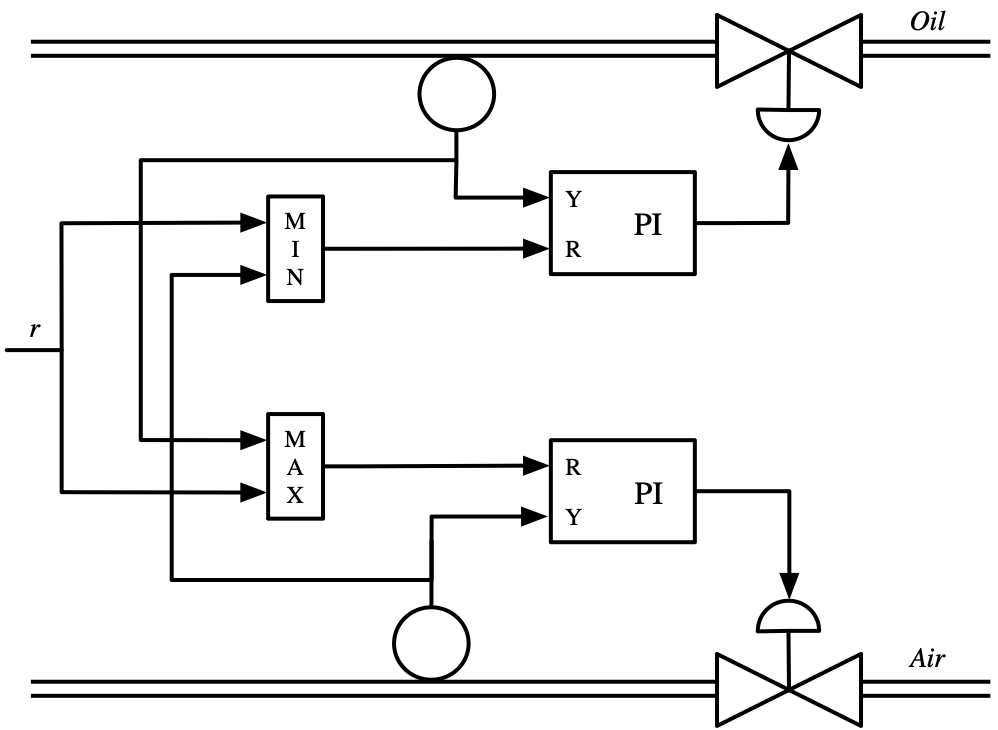
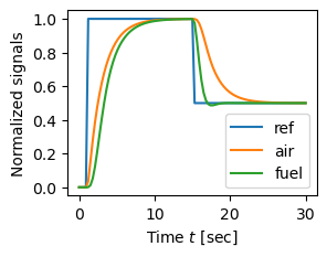
Figure 1.18: Air–fuel controller based on selectors
Jump to navigation
Jump to search
| Chapter | Introduction |
|---|---|
| Figure number | 1.18 |
| Figure title | Air–fuel controller based on selectors |
| GitHub URL | https://github.com/murrayrm/fbs2e-python/blob/main/figure-1.18-airfuel selectors.py |
| Requires | python-control |
Figure 1.18: Air–fuel controller based on selectors. The left figure shows the system architecture. The letters R and Y in the PI controller denote the input ports for reference and measured signal respectively. The right figure shows a simulation where the power reference r is changed stepwise at t = 1 and t = 15. Notice that the normalized air flow is larger than the normalized fuel flow both for increasing and decreasing reference steps.
# figure-1.18-airfuel_selectors.py - Air-fuel control example
# RMM, 20 Jun 2021
#
# Air–fuel controller based on selectors.  The right figure shows a
# simulation where the power reference r is changed stepwise at t = 1 and t
# = 15. Notice that the normalized air flow is larger than the normalized
# fuel flow both for increasing and decreasing reference steps.

# Package import
import numpy as np
import matplotlib.pyplot as plt
import control as ct
import cruise

#
# Air and fuel (oil) dynamics and controllers
#
# These dynamics come from Karl Astrom and are embedded in a SIMULINK
# diagram used for the initial part of the book.  The basic structure for
# both the air and fuel controllers is a PI controller with output feedback
# for the proportional term and integral feedback on the error.  This cuts
# the feedthrough term for the proportional feedback and gives a smoother
# step response (see Figure 11.1b for the basic structure).
#

# Min selector for oil PI controller input
min_block = ct.NonlinearIOSystem(
    updfcn=None, outfcn=lambda t, x, u, params: min(u),
    name='min', inputs=['u1', 'u2'], outputs='y')

# Max selector for air PI controller input
max_block = ct.NonlinearIOSystem(
    updfcn=None, outfcn=lambda t, x, u, params: max(u),
    name='max', inputs=['u1', 'u2'], outputs='y')

# Oil and air flow dynamics (from KJA SIMULINK diagram)
Po = ct.tf([1], [1, 1])
Pa = ct.tf([4], [1, 4])

# PI controller for oil flow
kpo = 2; kio = 4
Cio = ct.tf([kio], [1, 0])
Cpo = kpo
oil_block = ct.LinearIOSystem(
    ct.tf2ss(Po * Cio / (1 + Po * (Cio + Cpo))),
    name="oil", inputs='r', outputs='y')

# PI controller for air flow
kpa = 1; kia = 1
Cia = ct.tf([kia], [1, 0])
Cpa = kpa
air_block = ct.LinearIOSystem(
    ct.tf2ss(Pa * Cia / (1 + Pa * (Cia + Cpa))),
    name="air", inputs='r', outputs='y')

#
# Air-fuel selector dynamics
#
# The selector dynamics are based on the diagram Figure 1.18a, where we have
# already pre-computing the transfer function around the process/controller
# pairs (so the air and oil blocks have input 'R' and output 'Y' from the
# diagram).  We use the interconnect function along with named signals to
# set everything up.
#

airfuel = ct.interconnect(
    [min_block, max_block, oil_block, air_block],
    connections = (
        ['oil.r', 'min.y'],
        ['air.r', 'max.y'],
        ['min.u2', 'air.y'],
        ['max.u1', 'oil.y']),
    inplist = [['min.u1', 'max.u2']], inputs='ref',
    outlist = ['air.y', 'oil.y'], outputs=['air', 'oil'])

#
# Input/output response
#
# Finally, we simulate the dynamics with an input singla as showin in Figure
# 1.18b, consisting of a step increase from 0 to 1 at time t = 1 sec and
# then a decrease from 1 to 0.5 at time t = 15 sec.
#

T = np.linspace(0, 30, 101)
ref = np.array([
    0 if t <= 1 else
    1 if t <= 15 else
    0.5 for t in T])
t, y = ct.input_output_response(airfuel, T, ref)

# Plot the results
plt.subplot(2, 2, 1)
plt.plot(t, ref, t, y[0], t, y[1])

plt.legend(['ref', 'air', 'fuel'])
plt.xlabel('Time $t$ [sec]')
plt.ylabel('Normalized signals')

