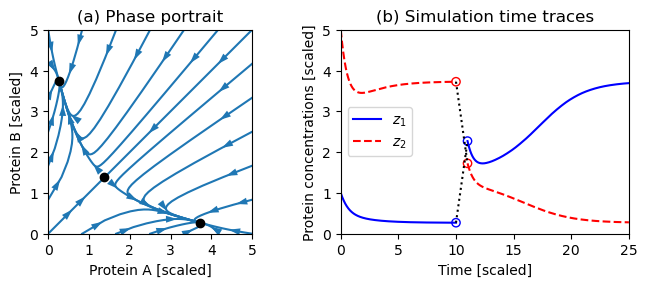
Figure 5.16: Dynamics of a genetic switch
Jump to navigation
Jump to search
| Chapter | Dynamic Behavior |
|---|---|
| Figure number | 5.16 |
| Figure title | Dynamics of a genetic switch |
| GitHub URL | https://github.com/murrayrm/fbs2e-python/blob/main/example-5.13-genetic switch.py |
| Requires | python-control |
Figure 5.16: Dynamics of a genetic switch. The phase portrait on the left shows that the switch has three equilibrium points, corresponding to protein A having a concentration greater than, equal to, or less than protein B. The equilibrium point with equal protein concentrations is unstable, but the other equilibrium points are stable. The simulation on the right shows the time response of the system starting from two different initial conditions. The initial portion of the curve corresponds to initial concentrations and converges to the equilibrium point where . At time , the concentrations are perturbed by +2 in and −2 in , moving the state into the region of the state space whose solutions converge to the equilibrium point where .
# example-5.13-genetic_switch.py - Genetic switch dynamics
# RMM, 17 Nov 2024
#
# Figure 5.15: Stability of a genetic switch. The circuit diagram in (a)
# represents two proteins that are each repressing the production of the
# other. The inputs u1 and u2 interfere with this repression, allowing the
# circuit dynamics to be modified. The equilibrium points for this circuit
# can be determined by the intersection of the two curves shown in (b).
#
# Figure 5.16: Dynamics of a genetic switch. The phase portrait on the left
# shows that the switch has three equilibrium points, corresponding to
# protein A having a concentration greater than, equal to, or less than
# protein B. The equilibrium point with equal protein concentrations is
# unstable, but the other equilibrium points are stable. The simulation on
# the right shows the time response of the system starting from two
# different initial conditions. The initial portion of the curve
# corresponds to initial concentrations z(0) = (1, 5) and converges to the
# equilibrium point where z1e < z2e. At time t = 10, the concentrations are
# perturbed by +2 in z1 and −2 in z2, moving the state into the region of
# the state space whose solutions converge to the equilibrium point where
# z2e < z1e.


import control as ct
import numpy as np
import matplotlib.pyplot as plt
from scipy.integrate import solve_ivp
from scipy.optimize import fsolve
ct.use_fbs_defaults()

#
# System dynamics
#

# Switch parameters
genswitch_params = {'mu': 4, 'n': 2}

def genswitch_dynamics(t, x, u, params):
    mu = params.get('mu')
    n = params.get('n')
    z1, z2 = x
    dz1 = mu / (1 + z2**n) - z1
    dz2 = mu / (1 + z1**n) - z2
    return [dz1, dz2]

genswitch_model = ct.nlsys(
    genswitch_dynamics, None, states=2, inputs=None, params=genswitch_params)

#
# 5.16 (a) Phase portrait
#

fig = plt.figure(constrained_layout=True)
gs = fig.add_gridspec(2, 2)
ax = fig.add_subplot(gs[0, 0])  # first row, first column

ct.phase_plane_plot(
    genswitch_model, [0, 5, 0, 5], 10, gridspec=[7, 7], ax=ax,
    plot_separatrices=False)

ax.axis('scaled')
ax.axis([0, 5, 0, 5])
ax.set_xticks([0, 1, 2, 3, 4, 5])       # defaults are different than y axis (?)
ax.set_xlabel("Protein A [scaled]")
ax.set_ylabel("Protein B [scaled]")
ax.set_title('(a) Phase portrait')

#
# 5.16 (b) Time traces
#

ax = fig.add_subplot(gs[0, 1])  # first row, second column

# Solve the ODE for the first segment
sol1 = ct.input_output_response(
    genswitch_model, np.linspace(0, 10, 1000), 0, [1, 5])

# Solve the ODE for the second segment
sol2 = ct.input_output_response(
    genswitch_model, np.linspace(11, 25, 1000), 0,
    [sol1.states[0, -1] + 2, sol1.states[1, -1] - 2])

# Second plot: Time traces
ax.plot(sol1.time, sol1.outputs[0], 'b-', label='$z_1$')
ax.plot(sol1.time, sol1.outputs[1], 'r--', label='$z_2$')
ax.plot(sol2.time, sol2.outputs[0], 'b-')
ax.plot(sol2.time, sol2.outputs[1], 'r--')
ax.plot(
    [sol1.time[-1], sol2.time[0]], [sol1.outputs[0, -1], sol2.outputs[0, -0]],
    'k:')
ax.plot(
    [sol1.time[-1], sol2.time[0]], [sol1.outputs[1, -1], sol2.outputs[1, -0]],
    'k:')
ax.scatter(
    [sol1.time[-1], sol2.time[0]], [sol1.outputs[0, -1], sol2.outputs[0, 0]],
    edgecolors='b', facecolors='none', marker='o')
ax.scatter(
    [sol1.time[-1], sol2.time[0]], [sol1.outputs[1, -1], sol2.outputs[1, 0]],
    edgecolors='r', facecolors='none', marker='o')
ax.axis([0, 25, 0, 5])
ax.set_xlabel('Time [scaled]')
ax.set_ylabel('Protein concentrations [scaled]')
ax.legend()
ax.set_title('(b) Simulation time traces')

# Save the second figure
plt.savefig("figure-5.16-genswitch_dynamics.png", bbox_inches='tight')


