Difference between revisions of "Figure 6.1: Superposition of homogeneous and particular solutions"
(Created page with "{{Figure |Chapter=Linear Systems |Figure number=6.1 |Sort key=601 |Figure title=Superposition of homogeneous and particular solutions |GitHub URL=https://github.com/murrayrm/f...") |
|||
| Line 11: | Line 11: | ||
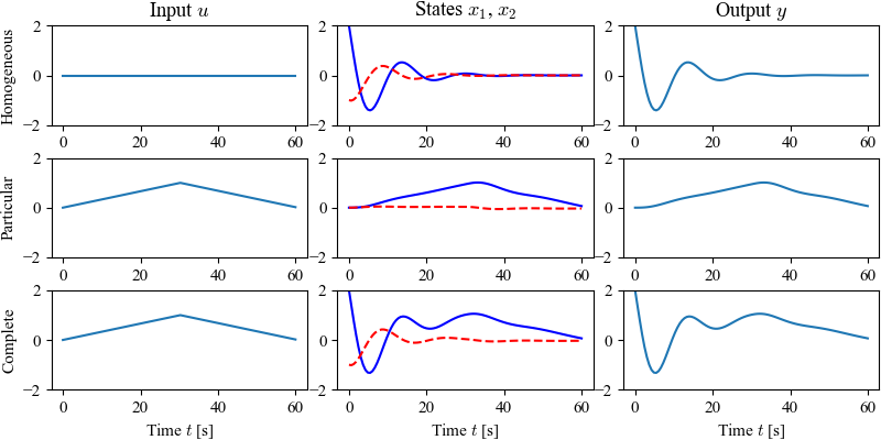
'''Figure65.1''': Superposition of homogeneous and particular solutions. The first row shows the input, state, and output corresponding to the initial condition response. The second row shows the same variables corresponding to zero initial condition but nonzero input. The third row is the complete solution, which is the sum of the two individual solutions. | '''Figure65.1''': Superposition of homogeneous and particular solutions. The first row shows the input, state, and output corresponding to the initial condition response. The second row shows the same variables corresponding to zero initial condition but nonzero input. The third row is the complete solution, which is the sum of the two individual solutions. | ||
| − | + | <nowiki> | |
# superposition.py - superposition of homogeneous and particular solutions | # superposition.py - superposition of homogeneous and particular solutions | ||
# RMM, 19 Apr 2024 | # RMM, 19 Apr 2024 | ||
Revision as of 12:00, 19 April 2024
| Chapter | Linear Systems |
|---|---|
| Figure number | 6.1 |
| Figure title | Superposition of homogeneous and particular solutions |
| GitHub URL | https://github.com/murrayrm/fbs2e-python/blob/main/figure-6.1-superposition.py |
| Requires | python-control, springmass.py |
Figure65.1: Superposition of homogeneous and particular solutions. The first row shows the input, state, and output corresponding to the initial condition response. The second row shows the same variables corresponding to zero initial condition but nonzero input. The third row is the complete solution, which is the sum of the two individual solutions.
<nowiki>
- superposition.py - superposition of homogeneous and particular solutions
- RMM, 19 Apr 2024
import matplotlib.pyplot as plt import numpy as np import control as ct import fbs # FBS plotting customizations
- Spring mass system
from springmass import springmass # use spring mass dynamics sys = springmass / springmass(0) # normalize the response to 1 X0 = [2, -1] # initial condition
- Create input vectors
tvec = np.linspace(0, 60, 100) u1 = 0 * tvec u2 = np.hstack([tvec[0:50]/tvec[50], 1 - tvec[0:50]/tvec[50]])
- Run simulations for the different cases
homogeneous = ct.forced_response(sys, tvec, u1, X0=X0) particular = ct.forced_response(sys, tvec, u2) complete = ct.forced_response(sys, tvec, u1 + u2, X0=X0)
- Plot results
fig, axs = plt.subplots(3, 3, figsize=[8, 4], layout='tight') for i, resp in enumerate([homogeneous, particular, complete]):
   axs[i, 0].plot(resp.time, resp.inputs)
   axs[0, 0].set_title("Input $u$")
   axs[i, 0].set_ylim(-2, 2)

   axs[i, 1].plot(
       resp.time, resp.states[0], 'b',
       resp.time, resp.states[1], 'r--')
   axs[0, 1].set_title("States $x_1$, $x_2$")
   axs[i, 1].set_ylim(-2, 2)
   axs[i, 2].plot(resp.time, resp.outputs)
   axs[0, 2].set_title("Output $y$")
   axs[i, 2].set_ylim(-2, 2)
- Label the plots
axs[0, 0].set_ylabel("Homogeneous") axs[1, 0].set_ylabel("Particular") axs[2, 0].set_ylabel("Complete") for i in range(3):
axs[2, i].set_xlabel("Time $t$ [s]")
- Save the figure
fbs.savefig('figure-6.1-superposition.png') <nowiki>
