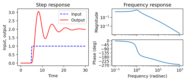
Figure 3.4: Input/output response of a linear system
Jump to navigation
Jump to search
| Chapter | System Modeling |
|---|---|
| Figure number | 4 |
| Figure title | Input/output response of a linear system |
| GitHub URL | https://github.com/murrayrm/fbs2e-python/blob/main/figure-3.4-io response.py |
| Requires | python-control |
Figure 3.2: Input/output response of a linear system. The step response (a) shows the output of the system due to an input that changes from 0 to 1 at time t = 5 s. The frequency response (b) shows the amplitude gain and phase change due to a sinusoidal input at different frequencies.
# figure-3-1-io_response.py - input/output response of a linear system
# RMM, 28 Aug 2021
#
# Figure 3.4: Input/output response of a linear system. The step
# response (a) shows the output of the system due to an input that
# changes from 0 to 1 at time t = 5 s. The frequency response (b)
# shows the amplitude gain and phase change due to a sinusoidal input
# at different frequencies.
#

import numpy as np
import scipy as sp
import matplotlib.pyplot as plt
import control as ct
ct.use_fbs_defaults()           # Use settings to match FBS

# System definition - third order, state space system
A = [[-0.2, 2, 0], [-0.5, -0.2, 4], [0, 0, -10]]
B = [0, 0, 1]
C = [2.6, 0, 0]
sys = ct.ss(A, B, C, 0)         # state space object

# Set up the plotting grid to match the layout in the book
fig = plt.figure(constrained_layout=True)
gs = fig.add_gridspec(4, 2)

#
# (a) Step response showing the output of the system due to an input
# that changes from 0 to 1 at time t = 5 s
#

fig.add_subplot(gs[0:2, 0])     # first column

# Create an input signal that is zero until time t = 5
t = np.linspace(0, 30, 100)
u = np.ones_like(t)
u[t < 5] = 0

# Compute the response
response = ct.forced_response(sys, t, u)
y = response.outputs

# Plot the response
plt.plot(t, u, 'b--', label="Input")
plt.plot(t, y, 'r-', label="Output")
plt.xlabel("Time (sec)")
plt.ylabel("Input, output")
plt.title("Step response")
plt.legend()

#
# (b) Frequency` response showing the amplitude gain and phase change
# due to a sinusoidal input at different frequencies
#

# Set up the axes for plotting (labels are recognized by bode_plot())
mag = fig.add_subplot(gs[0, 1], label='control-bode-magnitude')
phase = fig.add_subplot(gs[1, 1], label='control-bode-phase')

# Generate the Bode plot
ct.bode_plot(sys)

# Adjust the appearance to match the book
mag.xaxis.set_ticklabels([])
mag.set_title("Frequency response")
