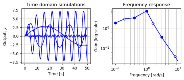
Figure 3.12: Frequency response computed by measuring the response of individual sinusoids

Chapter	System Modeling
Figure number	12
Figure title	A frequency response (gain only) computed by measuring # the response of individual sinusoids
GitHub URL	https://github.com/murrayrm/fbs2e-python/blob/main/figure-3.12-frequency response.py
Requires	python-control

Figure 3.12: A frequency response (gain only) computed by measuring the response of individual sinusoids. The figure on the left shows the response of the system as a function of time to a number of different unit magnitude inputs (at different frequencies). The figure on the right shows this same data in a different way, with the magnitude of the response plotted as a function of the input frequency. The filled circles correspond to the particular frequencies shown in the time responses.

# figure-3.12-frequency_response.py - frequency response computed by simulation
#
# Figure 3.12: A frequency response (gain only) computed by measuring
# the response of individual sinusoids.  The figure on the left shows
# the response of the system as a function of time to a number of
# different unit magnitude inputs (at different frequencies).  The
# figure on the right shows this same data in a different way, with
# the magnitude of the response plotted as a function of the input
# frequency. The filled circles correspond to the particular
# frequencies shown in the time responses.
#

import numpy as np
import matplotlib.pyplot as plt
import control as ct
ct.use_fbs_defaults()

# System definition - third order, state space system
A = [[-0.2, 2, 0], [-0.5, -0.2, 4], [0, 0, -10]]
B = [0, 0, 1]
C = [2.6, 0, 0]
sys = ct.ss(A, B, C, 0) * 1.4   # state space object (with tweaked scale)

# Set up the plotting grid to match the layout in the book
fig = plt.figure(constrained_layout=True)
gs = fig.add_gridspec(2, 2)

#
# (a) The response of the system as a function of time to a number of
# different unit magnitude inputs (at different frequencies).  
#

fig.add_subplot(gs[0, 0])       # first row, first column

# List of frequencies for the time simulations (and frequency response points)
omega_time = [0.1, 0.4, 1, 3]
mag_time = []                   # list to store magnitude of responses

# Manual computation of the frequency response
for omega in omega_time:
    # Compute out the time vector and inputs
    t = np.linspace(0, 50, 1000)
    u = np.sin(omega * t)

    # Simulate the system
    response = ct.forced_response(sys, t, u)

    # Plot the output
    plt.plot(response.time, response.outputs, 'b-')

    # Compute the magnitude of the response (avoiding initial transient)
    mag_time.append(max(response.outputs[500:]))

# Add grid lines
plt.xticks([0, 10, 20, 30, 40, 50])
plt.grid(which='major')

# Label the plot
plt.xlabel("Time [s]")
plt.ylabel("Output, $y$")
plt.title("Time domain simulations")

#
# (b) The same data in a different way, with the magnitude of the
# response plotted as a function of the input frequency. The filled
# circles correspond to the particular frequencies shown in the time
# responses.
#

fig.add_subplot(gs[0, 1])       # first row, second column

# List of frequencies to compute the frequency response
omega_freq = [0.1, 0.2, 0.4, 1, 1.6, 3, 8, 10]
mark_index = [1, 4, 6]          # frequencies to mark on the plot
mag_freq = []                   # list to store magnitude of responses

# Manual computation of the frequency response
for omega in omega_freq:
    # Compute out the time vector and inputs
    t = np.linspace(0, 50, 1000)
    u = np.sin(omega * t)

    # Simulate the system
    response = ct.forced_response(sys, t, u)

    # Compute the magnitude of the response (avoiding initial transient)
    mag_freq.append(max(response.outputs[500:]))

# Figure out which frequency points to mark
omega_mark = np.array(omega_freq)[mark_index]
mag_mark = np.array(mag_freq)[mark_index]

# Plot the results
plt.loglog(omega_freq, mag_freq, 'b-')
plt.loglog(omega_mark, mag_mark, 'bo', markerfacecolor='none')
plt.loglog(omega_time, mag_time, 'bo')

plt.grid(axis='x', which='minor')
plt.grid(axis='y', which='major')

# Label the plot
plt.xlabel("Frequency [rad/s]")
plt.ylabel("Gain (log scale)")
plt.title("Frequency response")

plt.savefig("figure-3.12-frequency_response.png", bbox_inches='tight')