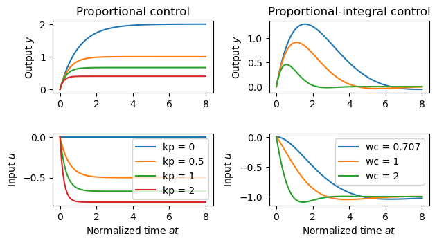
Figure 2.8: Step responses for a first-order, closed loop system with proportional and PI control

Chapter	Feedback Principles
Figure number	2.8
Figure title	Step responses for a first-order, closed loop system with proportional # control and PI control.
GitHub URL	https://github.com/murrayrm/fbs2e-python/blob/main/figure-2.8-PI step responses.py
Requires	python-control

Figure 2.8: Step responses for a first-order, closed loop system with proportional control (a) and PI control (b). The process transfer function is $P = 2/(s + 1)$. The controller gains for proportional control are $k_p = $$, 0.5, 1, and 2. The PI controller is designed using equation (2.28) with $\zeta_c = 0.707$ and $\omega_c = 0.707$$, 1, and 2, which gives the controller parameters $k_p = 0$, 0.207, and 0.914 and $k_i = 0.25$, 0.50, and 2.

# figure-2.8-PI_step_reesponses.py - step responses for P/PI controllers
# RMM, 21 Jun 2021
#
# Step responses for a first-order, closed loop system with proportional
# control and PI control. The process transfer function is P = 2/(s + 1).
# The controller gains for proportional control are k_p = 0, 0.5, 1, and
# 2. The PI controller is designed using equation (2.28) with zeta_c = 0.707
# and omega_c = 0.707, 1, and 2, which gives the controller parameters k_p =
# 0, 0.207, and 0.914 and k_i = 0.25, 0.50, and 2.
#

import numpy as np
import matplotlib.pyplot as plt
import control as ct

# Process model
b = 2; a = 1
P = ct.tf([b], [1, a])

# Set the simulation time vector
time = np.linspace(0, 8, 100)

#
# Proportional control
#

# Choose gains to use
kp_gains = [0, 0.5, 1, 2]

for kp in kp_gains:
    Gyv = ct.tf([b], [1, a + b*kp])
    Guv = ct.tf([-b*kp], [1, a + b*kp], dt=0)   # force kp=0 to be cts time

    t, y = ct.step_response(Gyv, time)
    t, u = ct.step_response(Guv, time)

    if 'p_y_ax' not in locals():
        p_y_ax = plt.subplot(3, 2, 1)
        plt.ylabel('Output $y$')
        plt.title('Proportional control')
    p_y_ax.plot(t, y)

    if 'p_u_ax' not in locals():
        p_u_ax = plt.subplot(3, 2, 3)
        plt.ylabel('Input $u$')
        plt.xlabel('Normalized time $at$')
    p_u_ax.plot(t, u, label="kp = %0.3g" % kp)

# Label proportional control curves
p_u_ax.legend()

#
# PI control
#

# Figure out frequency of critical damping
zeta = 0.707
wc = a / 2 / zeta 

# Plot results for different resonate frequencies
wc_list = [wc, 1, 2]
for wc in wc_list:
    kp = (2 * zeta * wc - a) / b
    ki = wc**2 / b
    
    Gyv = ct.tf([b, 0], [1, a + b*kp, b*ki])
    Guv = -ct.tf([b*kp, b*ki], [1, a + b*kp, b*ki], dt=0)

    t, y = ct.step_response(Gyv, time)
    t, u = ct.step_response(Guv, time)

    if 'pi_y_ax' not in locals():
        pi_y_ax = plt.subplot(3, 2, 2)
        plt.ylabel('Output $y$')
        plt.title('Proportional-integral control')
    pi_y_ax.plot(t, y)

    if 'pi_u_ax' not in locals():
        pi_u_ax = plt.subplot(3, 2, 4)
        plt.ylabel('Input $u$')
        plt.xlabel('Normalized time $at$')
    pi_u_ax.plot(t, u, label="wc = %0.3g" % wc)

# Label PI curves
pi_u_ax.legend()

# Overalll figure labeling
plt.tight_layout()