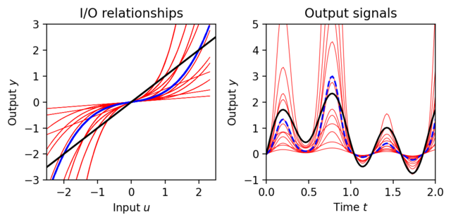
Figure 2.12: Responses of a static nonlinear system
Jump to navigation
Jump to search
| Chapter | Feedback Principles |
|---|---|
| Figure number | 12 |
| Figure title | Responses of a static nonlinear system |
| GitHub URL | https://github.com/murrayrm/fbs2e-python/blob/main/figure-2.12,14-static nlsys.py |
| Requires | python-control |
Figure 2.12: Responses of a static nonlinear system. The left figure shows the input/output relations of the open loop systems and the right figure shows responses to the input signal (2.38). The ideal response is shown with solid bold lines. The nominal response of the nonlinear system is shown using dashed bold lines and the responses for different parameter values are shown using thin lines. Notice the large variability in the responses.
# figure-2.12,14-static_nlsys.py - static nonlinear feedback system
# RMM, 21 Jun 2021
#
# Figure 2.12: Responses of a static nonlinear system. The left figure shows
# the in- put/output relations of the open loop systems and the right figure
# shows responses to the input signal (2.38). The ideal response is shown
# with solid bold lines. The nominal response of the nonlinear system is
# shown using dashed bold lines and the responses for different parameter
# values are shown using thin lines. Notice the large variability in the
# responses.
#
# Figure 2.14: Responses of the systems with integral feedback (ki =
# 1000). The left figure shows the input/output relationships for the closed
# loop systems, and the center figure shows responses to the input signal
# (2.38) (compare to the corresponding responses in Figure 2.12. The right
# figure shows the individual errors (solid lines) and the approximate error
# given by equation (2.42) (dashed line).
#
# Intial code contributed by Adam Matic, 26 May 2021.
#

import numpy as np
import matplotlib.pyplot as plt
import control as ct

# Static nonlinearity
def F(u, alpha, beta):
    return alpha * (u + beta * (u ** 3))

# Reference signal
t = np.linspace(0, 6, 300)
r = np.sin(t) + np.sin(np.pi * t) + np.sin((np.pi**2) * t)

#
# Open loop response
#

# Set up the plots for Figure 2.12
fig, [ax1, ax2] = plt.subplots(1, 2, figsize=(6, 3))

# Generate the input/output curves and system responses
for a in [0.1, 0.2, 0.5]:
    for b in [0, 0.5, 1, 2]:
        y = F(r, a, b)
        ax1.plot(r, y, 'r', linewidth=0.5);
        ax2.plot(t, y, 'r', linewidth=0.5)

# Generate the nominal response
y = F(r, 0.2, 1)
ax1.plot(r, y, 'b--', linewidth=1.5);
ax2.plot(t, y, 'b--', linewidth=1.5)

# Left plot labels
ax1.set_title("I/O relationships")
ax1.set_xlabel("Input $u$")
ax1.set_ylabel("Output $y$")

# Draw reference line, set axis limits
ax1.plot(y, y, 'k-', linewidth=1.5)
ax1.set_ylim(-3, 3)
ax1.set_xlim(-2.5, 2.5)

# Right plot labels
ax2.set_title("Output signals")
ax2.set_xlabel("Time $t$")
ax2.set_ylabel("Output $y$")

# Draw reference line, set axis limits
ax2.plot(t, r, 'k-', linewidth=1.5)
ax2.set_ylim(-1, 5)
ax2.set_xlim(0, 2)

plt.tight_layout()
