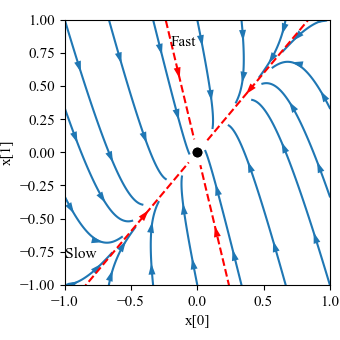
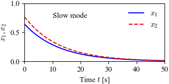
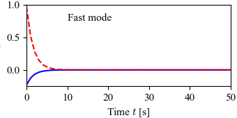
Figure 6.5: Modes for a second-order system with real eigenvalues

Chapter	Linear Systems
Figure number	6.5
Figure title	Figure 6.5: The notion of modes for a second-order system with real eigenvalues.
GitHub URL	https://github.com/murrayrm/fbs2e-python/blob/main/figure-6.5-springmass modes.py
Requires	python-control, springmass.py

Figure 5.1: Response of the damped oscillator to the initial condition x0 = (1, 0). The solution is unique for the given initial conditions and consists of an oscillatory solution for each state, with an exponentially decaying magnitude.

{| border=0
|-
| rowspan=2 | [[Image:figure-6.5-modes-pp.png]] 
| [[Image:figure-6.5-modes-slow.png]] 
|-
| [[Image:figure-6.5-modes-fast.png]] 
|}

'''Figure 5.1''': Response of the damped oscillator to the initial condition x0 = (1, 0). The solution is unique for the given initial conditions and consists of an oscillatory solution for each state, with an exponentially decaying magnitude.

 <nowiki>
# modes.py - illustration of modes for a second order system
# RMM, 19 Apr 2024

import matplotlib.pyplot as plt
import numpy as np
import control as ct
import fbs                      # FBS plotting customizations

# System definition
k0, k1, k2, b0 = 0.1, 0.1, 0.5, 1.5
A = [[-k0 - k1, k1], [k2, -k2]]
B = [[b0], [0]]
C = [[1, 0], [0, 1]]
sys = ct.ss(A, B, C, 0)

# Generate a phase plot for the system
fig, ax = plt.subplots(1, 1, figsize=[3.4, 3.4])
ct.phase_plane_plot(sys, [-1, 1, -1, 1], 5, gridspec=[7, 4])
ax.set_aspect('equal')

# Label the figure
plt.suptitle("")
plt.text(-1, -0.8, "Slow")
plt.text(-0.2, 0.8, "Fast")
fbs.savefig('figure-6.5-modes-pp.png')

# Time domain simulations
evals, evecs = np.linalg.eig(A)
X0s, X0f = evecs[:, 0], evecs[:, 1]   # Fast and slow modes
tvec = np.linspace(0, 50, endpoint=True)

# Slow mode
ax = fbs.figure('321')
resp_slow = ct.initial_response(sys, tvec, X0=X0s)

ax.set_xlim([0, 50])
ax.set_ylim([0, 1])
ax.plot(tvec, resp_slow.states[0], 'b', label="$x_1$")
ax.plot(tvec, resp_slow.states[1], 'r--', label="$x_2$")
ax.text(10, 0.75, "Slow mode")
ax.set_xlabel("Time $t$ [s]")
ax.set_ylabel("$x_1, x_2$")
ax.legend(frameon=False)

plt.tight_layout()
fbs.savefig('figure-6.5-modes-slow.png')

# Fast mode
ax = fbs.figure('321')
resp_fast = ct.initial_response(sys, tvec, X0=X0f)

ax.set_xlim([0, 50])
ax.set_ylim([-0.25, 1])
ax.plot(tvec, resp_fast.states[0], 'b', label="$x_1$")
ax.plot(tvec, resp_fast.states[1], 'r--', label="$x_2$")
ax.text(10, 0.75, "Fast mode")
ax.set_xlabel("Time $t$ [s]")
ax.set_ylabel("$x_1, x_2$")

plt.tight_layout()
fbs.savefig('figure-6.5-modes-fast.png')