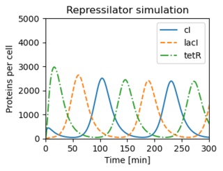
Figure 3.26: The repressilator genetic regulatory network

Chapter	System Modeling
Figure number	3.26
Figure title	The repressilator genetic regulatory network
GitHub URL	https://github.com/murrayrm/fbs2e-python/blob/main/example-3.18-repressilator.py
Requires	python-control

Figure 3.26: The repressilator genetic regulatory network. (b) A simulation of a simple model for the repressilator, showing the oscillation of the individual protein concentrations.

# example-3.18-repressilator.py - Transcriptional regulation
# RMM, 29 Aug 2021
#
# Figure 3.26: The repressilator genetic regulatory network. (a) A schematic
# diagram of the repressilator, showing the layout of the genes in the
# plasmid that holds the circuit as well as the circuit diagram
# (center). (b) A simulation of a simple model for the repressilator,
# showing the oscillation of the individual protein concentrations.
#

import control as ct
import numpy as np
import matplotlib.pyplot as plt

#
# Repressilator dynamics
#
# This function implements the basic model of the repressilator All
# parameter values were taken from Nature. 2000 Jan 20; 403(6767):335-8.
#
# This model was developed by members of the 2003 Synthetic Biology Class
# on Engineered Blinkers.
#

# Dynamics for the repressilator
def repressilator(t, x, u, params):
    # store the state variables under more meaningful names
    mRNA_cI = x[0]
    mRNA_lacI = x[1]
    mRNA_tetR = x[2]
    protein_cI = x[3]
    protein_lacI = x[4]
    protein_tetR = x[5]

    #
    # set the parameter values
    #

    # set the max transcription rate in transcripts per second
    k_transcription_cI = params.get('k_transcription_cI', 0.5)
    k_transcription_lacI = params.get('k_transcription_lacI', 0.5)
    k_transcription_tetR = params.get('k_transcription_tetR', 0.5)

    # set the leakage transcription rate (ie transcription rate if
    # promoter region bound by repressor) in transcripts per second
    k_transcription_leakage = params.get('k_transcription_leakage', 5e-4)

    # Set the mRNA and protein degradation rates (per second)
    mRNA_half_life = params.get('mRNA_half_life', 120)          # in seconds
    k_mRNA_degradation = np.log(2)/mRNA_half_life
    protein_half_life = params.get('protein_half_life', 600)    # in seconds
    k_protein_degradation = np.log(2)/protein_half_life

    # proteins per transcript lifespan
    translation_efficiency = params.get('translation_efficiency', 20)
    average_mRNA_lifespan = 1/k_mRNA_degradation

    # proteins per transcript per sec
    k_translation = translation_efficiency/average_mRNA_lifespan 

    # set the Hill coefficients of the repressors
    n_tetR = params.get('n_tetR', 2)
    n_cI = params.get('n_cI', 2)
    n_lacI = params.get('n_lacI', 2)

    # Set the dissociation constant for the repressors to their target promoters
    # in per molecule per second
    KM_tetR = params.get('KM_tetR', 40)
    KM_cI = params.get('KM_cI', 40)
    KM_lacI = params.get('KM_lacI', 40)

    # the differential equations governing the state variables:
    # mRNA concentration = transcription given repressor concentration - 
    # mRNA degradation + transcription leakage
    dxdt = np.empty(6)
    dxdt[0] = k_transcription_cI/(1 + (protein_tetR / KM_tetR) ** n_tetR) - \
        k_mRNA_degradation * mRNA_cI + k_transcription_leakage
    dxdt[1] = k_transcription_lacI/(1 + (protein_cI / KM_cI)**n_cI) - \
        k_mRNA_degradation * mRNA_lacI + k_transcription_leakage
    dxdt[2] = k_transcription_tetR/(1 + (protein_lacI / KM_lacI) ** n_lacI) - \
        k_mRNA_degradation * mRNA_tetR + k_transcription_leakage

    # protein concentration = translation - protein degradation
    dxdt[3] = k_translation*mRNA_cI - k_protein_degradation*protein_cI
    dxdt[4] = k_translation*mRNA_lacI - k_protein_degradation*protein_lacI
    dxdt[5] = k_translation*mRNA_tetR - k_protein_degradation*protein_tetR

    return dxdt

# Define the system as an I/O system
sys = ct.NonlinearIOSystem(
    updfcn=repressilator, outfcn=lambda t, x, u, params: x[3:],
    states=6, inputs=0, outputs=3)

# Set up the plotting grid to match the layout in the book
fig = plt.figure(constrained_layout=True)
gs = fig.add_gridspec(2, 2)

#
# (b) A simulation of a simple model for the repressilator, showing the
# oscillation of the individual protein concentrations.
#

fig.add_subplot(gs[0, 1])       # first row, second column

# Initial conditions and time
t = np.linspace(0, 20000, 1000)
x0 = [1, 0, 0, 200, 0, 0]

# Integrate the differential equation
response = ct.input_output_response(sys, t, 0, x0)

# Plot the results (protein concentrations)
plt.plot(response.time/60, response.outputs[0], '-')
plt.plot(response.time/60, response.outputs[1], '--')
plt.plot(response.time/60, response.outputs[2], '-.')

plt.axis([0, 300, 0, 5000])
plt.legend(("cI", "lacI", "tetR"), loc='upper right')

plt.xlabel("Time [min]")                        # Axis labels
plt.ylabel("Proteins per cell")
plt.title("Repressilator simulation")           # Plot title

# Save the figure
plt.savefig("figure-3.26-repressilator_dynamics.png", bbox_inches='tight')